An introduction to Recommendation Systems: an overview of machine and deep learning architectures

Recommendation systems have become one of the most popular applications of machine learning in today’s websites and platforms. The rapid rise of eCommerce made personalized suggestions to clients a necessity in order for the e-store to distinguish itself. Nowadays, recommendation systems are at the core of online services such as Amazon, Netflix, Youtube, Spotify.

But what exactly is a recommendation system? According to Wikipedia:

A recommender system, or a recommendation system (sometimes replacing 'system' with a synonym such as a platform or an engine), is a subclass of information filtering system that seeks to predict the "rating" or "preference" a user would give to an item.

TL;DR

In this article, we will explore the most popular architectures from recommendation systems. We will start with primitive strategies such as collaborative and content-based filtering and we will continue with state-of-the-art deep learning-based methods

For a holistic approach to recommender systems we highly suggest the Recommender Systems Specialization by the University of Michigan.

Problem Formulation

In most cases, we start with a number of items (products, videos, songs, etc.). Each item has a set of characteristics/features that define it. Our goal is to build a model that predicts items that a user may have an interest in. There are many intuitive approaches to how we select this item. Popular ones include:

Based on their popularity
Based on the user’s previous interaction
Based on interactions of similar users

Or more often than not, based on a mixture of the above.

In most systems, we typically have a form of a score that we evaluate the item’s relevancy and some sort of feedback that we get from the users.

Now that we have a clear picture of the basics, let’s continue with the fundamental techniques.

Content-based filtering

Content-based filtering uses the similarity between items to recommend items similar to what a user likes.

Typically, each item with its features is mapped to a low-dimensional embedding space. Then, using a similarity measure, one can identify items in the same neighborhood on the embedding space and suggest those items to the users. The similarity function can be simple functions such as the dot-product, or the Euclidean distance, or more complex ones.

Mathematically we have:

Given a query item $q$ and a similarity measure $s(q,x)$ , the model will look for an item $x$ that is close to $q$ based on their similarity. For example:

Given a similarity measure $s(q,x) = \sqrt{\sum_{i=1}^N (q^i - x^i)^2}$ , a query item $q=[1, 4 ,5]$ and a set of items $(x_1,x_2,x_3 ) = ( [2, 3, 2 ] , [1, 0, 0 ] , [4, 5,1 ] )$ , the model will calculate the similarity of $q$ with all items and selects the one with the smaller.

$s(q,x_1) = 3.31$

$s(q,x_2) = 6.43$

$s(q,x_3) = 5.09$

So the model will recommend the first item to the user.

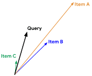Source: developers.google.com

Collaborative filtering

Collaborative filtering (CF) is a traditional approach that follows a simple principle: We should recommend items to a client based on the inputs or actions of other clients (preferably similar ones).

Let’s look at a simplistic example to demystify this sentence.

In the table below we see the interactions between 3 users and 5 items. Each user has given a rating on a scale [1,5] to each of the items he has used. We want to suggest an item to “user 3”

	User 1	User 2	User 3
Item 1	5	2	4
Item 2	3	4	3
Item 3	1	4	1
Item 4	2		?
Item 5	5	2	?

Memory-based CF

One approach is to look at similar users and recommend items that they like. This is called user-based CF. In the above table, we can see that users 1 and 3 have similar tastes in items (they both like item 1 and dislike item 3). So if we’d want to recommend an item to user 3, we would probably pick item 5 because user 1 seems to really like it.

A different approach is to find similar items based on ratings given by other users. This is called item-based CF. Since user 1 likes item 1, we need to find an item that other users have rated similarly. We can see that the ratings between item 1 and item 3 are very close so item 3 is a natural choice to recommend to user 3.

As we did in content-based systems, the similarity between users or items based on the ratings can be formulated using a similarity measure $s(q,x)$ . You can imagine that traditional machine learning methods such as k-Nearest Neighbors (k-NN) can be utilized here as well.

Both of the above approaches fall in the category of memory-based CF.

Model-based CF

Model-based CF tries to model the interaction matrix between items and users. Each user and item can be mapped into an embedding space based on their features.

The embeddings can be learned using a machine learning model so that close embeddings will correspond to similar items/users.

This brings us to the most important model for recommendation systems: Matrix Factorization. Matrix factorization falls into the category of model-based CF.

Matrix Factorization

In simple terms, Matrix Factorization (MF) algorithms work by decomposing the user-item interaction matrix into the product of two lower dimensionality rectangular matrices.

Suppose that we denote the interaction matrix $A \in R^{m \times n}$ , where $m$ is the number of users and $n$ the number of items. We also denote $U \in R^{m \times d}$ the user embedding matrix and $V \in R^{n \times d}$ the item embedding matrix.

Item and user embedding matrices $U$ and $V$ contain a compact representation of all items/users features respectively. The $i$ th row in $U$ gives us the embedding for the user $i$ , while the $j$ row in $V$ gives us the embedding for item $j$ .

The model tries to learn the matrices $U$ and $V$ so that $UV^T = A$ .

For example:

\begin{pmatrix} u_{11} & u_{12} & u_{13} \\ u_{21} & u_{22} & u_{23} \\ u_{31} & u_{32} & u_{33} \\ u_{41} & u_{42} & u_{43} \\ u_{51} & u_{52} & u_{53} \end{pmatrix} \cdot \begin{pmatrix} v_{11} & v_{12} & v_{13} & v_{14} \\ v_{21} & v_{22} & v_{23} & v_{34} \\ v_{31} & v_{32} & v_{33} & v_{44} \\ \end{pmatrix} = \begin{pmatrix} a_{11} & a_{12} & a_{13} & a_{14} \\ a_{21} & a_{22} & a_{23} & a_{24} \\ a_{31} & a_{32} & a_{33} & a_{34} \\ a_{41} & a_{42} & a_{43} & a_{44} \\ a_{51} & a_{52} & a_{53} & a_{54} \end{pmatrix}

Each element on the $A$ matrix corresponds to the interaction of a specific user with a specific item. In practice, we also introduce a set of biases $b_u$ and $b_v$ for users and items, respectively.

Many loss functions have been proposed over the years to train such models. The most simple one is the squared distance.

\min_{U,V} ||A - UV^T||^2

Once we have trained an MF model, we have a way to predict the interaction between a user and a model. So in order to recommend a new item to a user, we simply get all the “ratings” and return the highest one.

Nonetheless you have to consider the scaling of such methods for a huge number of items or users. And that brings us to...

Deep Learning-based Recommendation systems

Before we explore some state-of-the-art architectures, let’s discuss a few key ideas of deep learning-based methods. It’s undeniable that deep networks are excellent feature extractors and that’s why they are ideal for recommendation systems. Their ability to capture contextual information and generate user/item compact embeddings is unparalleled.

Deep Content-based recommendation

That’s why Deep Learning can be used for standard content-based recommendations. By using a neural network, we can construct high-quality low-dimensional embeddings and recommend items close in the embedding space. Spotify has used this approach with great success: they used a CNN to transform audio (in the form of mel spectrograms) into compact representations, and then suggest to the user similar songs with what they have already listened to.

This idea can be extended into content embeddings (Content2Vec) where we can represent all kinds of items in an embedding space; whether the items are images, text, songs etc. Then we use a pair-wise item similarity metric to generate recommendations. Transfer learning can obviously play a major role in this approach.

The content embeddings can be used either in a content-based strategy or as extra information on CF techniques, as we will see.

Candidate Generation and Ranking

One frequent idea on systems with a huge amount of items and users is to split the recommendation pipeline into two steps: candidate generation and ranking.

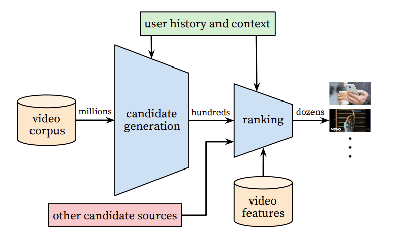Candidate generation and ranking pipeline. Source: Deep Neural Networks for YouTube Recommendations

Candidate generation: First we generate a larger set of relevant candidates based on our query using some approach. This step is called Retrieval in literature
Ranking: After candidate generation, another model ranks the candidates producing a list of the top N recommendations
Re-Ranking: In some implementations, we perform another round of ranking based on additional criteria in order to remove some irrelevant candidates.

As you may have imagined, the philosophy behind this is twofold:

To reduce the complexity of the systems by avoiding running the model into the entire dataset
To produce better and more relevant recommendations

Now it’s time to continue with the most popular methods for building large-scale recommendation systems. In some categories we’ll look at specific architectures and in others we’ll discuss a more general approach.

Let’s begin.

Wide and Deep Learning

Wide and Deep Networks were originally proposed by Google and is an effort to combine traditional linear models with deep models.

Shallow linear models are good at capturing and memorizing low-order interaction features, while deep networks are great at extracting high-level features.

Wide & Deep Learning for Recommender Systems

Wide and Deep models have proven to work very well for classification problems with sparse inputs such as recommender systems. Let’s take a closer look.

Wide models are generalized linear models with non-linear transformations and they are trained on a wide set of cross-product transformations. The goal is to memorize specific useful feature combinations. On the other hand, deep models are learning items and user embeddings, which makes them able to generalize in unseen pairs without manual feature engineering.

The fusion of wide and deep models combines the strengths of memorization and generalization, and provides us with better recommendation systems. The two models are trained jointly with the same loss function.

An example of wide and deep learning: movie recommendations

Let’s assume that we want to recommend movies to users (e.g. we’re building a system for Netflix). Intuitively we can think that wide models will memorize things such as: “Bob liked Terminator 2” or “Alice hated The Avengers”. Or the other hand, deep models will capture generic information such as: “Most teenage boys like action films” or “Middle-age women don’t like superhero movies”. The combination of these two helps us acquire better recommendations.

Deep Factorization Machines (DeepFm)

Deep Factorization Machines have gained a lot of popularity over the years. Before we analyze how they work, let’s first discuss simple Factorization Machines.

Factorization Machines (FM)

Factorization Machines is a generalized version of the linear regression model and the matrix factorization model. It improves upon them by supporting “n-way” variable interactions where $n$ is the polynomial degree of the model. Usually, we use a degree of 2 but higher ones are also possible. Note though that in higher-degree FM, the numerical instability and the computational complexity increases.

Mathematically we have:

\hat{y}(x) = \mathbf{w}_0 + \sum_{i=1}^d \mathbf{w}_i x_i + \sum_{i=1}^d\sum_{j=i+1}^d \langle\mathbf{v}_i, \mathbf{v}_j\rangle x_i x_j

where $\mathbf{w}_0$ is a global bias, $\mathbf{w}$ the weights of the i-th variable, $\mathbf{v}_i$ the i-th row of the features embeddings matrix $V$ , and $k$ the dimensionality of the feature embeddings.

It is obvious from the equation that the first two-terms correspond to the traditional linear regression. The last term corresponds to the matrix factorization model if we assume that $\mathbf{v}_i$ is a user embedding and $\mathbf{v}_j$ an item embedding. Their dot-product models their interaction (similarity).

DeepFM

Deep Factorization Machines (DeepFM) improve upon the aforementioned idea by using Deep Neural Networks. DeepFM consists of an FM component and a deep network.

The FM component is identical to the one mentioned in the FM section and aims to model low-order interactions between the features. The deep network is a standard MLP that, as you might have guessed, aims to model high-level interactions. I’m sure you noticed the similarity with Wide and Deep models. One might argue that DeepFM shares the same principles with them and this would be 100% correct.

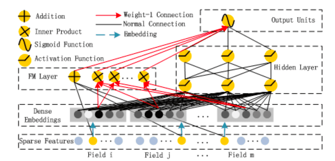DeepFM: A Factorization-Machine based Neural Network for CTR Prediction

The final prediction of the model is the summation from both subcomponents:

\hat{y} = \sigma(\hat{y}^{(FM)} + \hat{y}^{(DNN)})

Neural Collaborative Filtering

Neural Collaborative Filtering is an extension of CF that uses implicit feedback and neural networks.

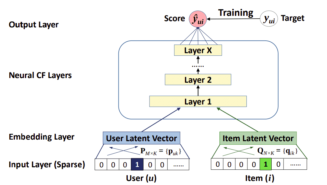Neural Collaborative Filtering framework. Source: Neural Collaborative Filtering

Implicit feedback is the feedback that the user doesn’t specifically give but is inherited from the user’s behavior. Examples include user actions, clicks, browsing history, search patterns, etc.

The most common model is called NeuMF, short for neural matrix factorization, and aims to replace standard matrix factorization with neural networks. Specifically, it consists of two submodels: A Generalized Matrix Factorization (GMF) model and a traditional MLP model.

The GMF is a neural network approach of matrix factorization where the input is an element-wise product of the user and item embeddings and the output is a prediction score that maps the interaction between the user and the item.

The MLP model serves as an extra layer on modeling the user-item interaction. It concatenates the user and item embeddings and through the addition of more non-linear layers, it models the collaborative filtering effect.

To fuse the two models, no embeddings were shared in fear of limiting the model’s capacity. Instead, NeuMF concatenates the second last layers of two subnetworks to create a final interaction score. This way, we can generate a ranked recommendation list for each user based on the implicit feedback.

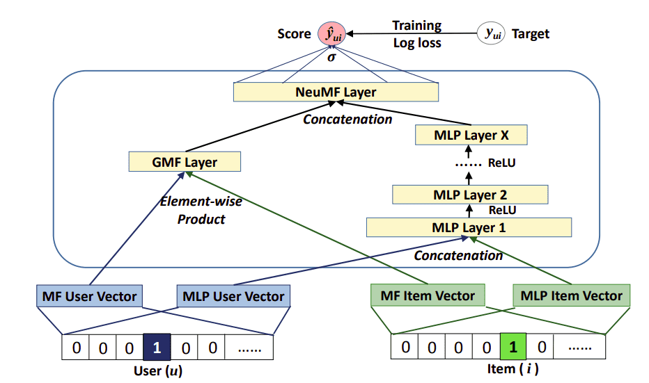NeuMF. Source: Neural Matrix Factorization model

Recommendation with Autoencoders

One very interesting idea is the utilization of Autoencoder in recommender systems. The most famous example is AutoRec, which extends the basic CF paradigm with the expressiveness of deep networks.

AutoRec follows the traditional architecture of Autoencoders in the sense that it tries to reconstruct its input. But with one key difference: It accepts only a single row/column of the interaction matrix as an input and then tries to reconstruct the entire interaction matrix.

Contrary to the traditional architecture, the end goal isn’t to find the compact latent representation of the input. Here we primarily care about its output: the interaction matrix between users and items. Note that here we only make use of explicit feedback.

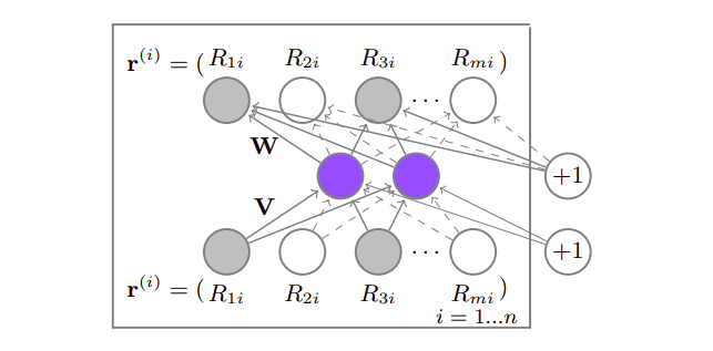AutoRec: Autoencoders Meet Collaborative Filtering

If we denote the reconstruction as $h(\mathbf{r},\theta)$ for input $\mathbf{r}$ , and $\mathbf{V}$ and $\mathbf{W}$ the weight matrices, and $f$ , $g$ the activation functions, we can represent the model’s architecture as:

h(\mathbf{r},\theta) = f(\mathbf{W} \cdot g(\mathbf{V} \mathbf{r} + \mu) + b)

where $\mu$ and $b$ are the networks’ biases.

The network is trained with a regularized reconstruction loss in the form of:

\underset{\theta}{\mathrm{min}} \sum_{i=1}^n{\parallel \mathbf{r}^{(i)} - h(\mathbf{r^{(i)}};\theta)\parallel_{\mathcal{O}}^2} +\frac{\lambda}{2}(\| \mathbf{W} \|_F^2 + \| \mathbf{V}\|_F^2)

where $\| \cdot \|_{\mathcal{O}}$ means that only the contribution of observed ratings are considered.

As a final note: AutoRec can be thought as modeling the matrix factorization algorithm with autoencoders

More Autoencoder-based systems include: DeepRec, Collaborative Denoising Auto-Encoders, Multinomial Variational Auto-encoder, Embarrassingly Shallow Autoencoders for Sparse Data

Sequence aware recommendation

Sequence aware recommendation aims to apply the advancements of sequence models in recommendation systems. Whether they are RNN-based or transformers-based architectures, most models follow the below framework:

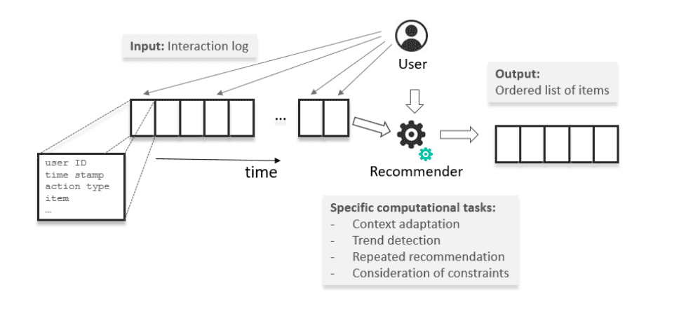High-level Overview of Sequence-Aware Recommendation Problems. Source: Sequence-Aware Recommender Systems

The input of sequence-aware recommendation systems is usually an ordered list of the user's past interactions. These interactions can be associated with specific items or not. The output is a ranked list of items in a similar way to most aforementioned strategies. Contextual information can also be added to the mix in the form of context embeddings.

Sequence aware systems can be divided into different categories:

Context-aware or not
Short-term or Long-term
Session-based or not

Sequence-aware systems can model the users behavior very effectively and in many cases outperform CF-based systems. A hybrid system consisting of both approaches usually works even better.

SOTA sequence-based models include: GRU4Rec, BERT4Rec, SASRec

Deep and Cross Network (DCN)

As we have already discussed, modeling interactions between features give us better recommendations compared to using single features. In bibliography, you may see the term cross-feature when talking about feature interactions.

A cross-feature is a combination of 2 or more features which provides additional interaction information beyond individual features. A combination of 2 individual features is a 2nd degree cross-feature.

Deep and Cross Network (DCN) is an architecture proposed by Google and is designed to learn explicit cross-features in an effective manner. As with many previous models, we have two submodules: The cross-network and the deep network. We can either stack the two networks on top of each other or combine their final prediction. The figure below follows the first approach.

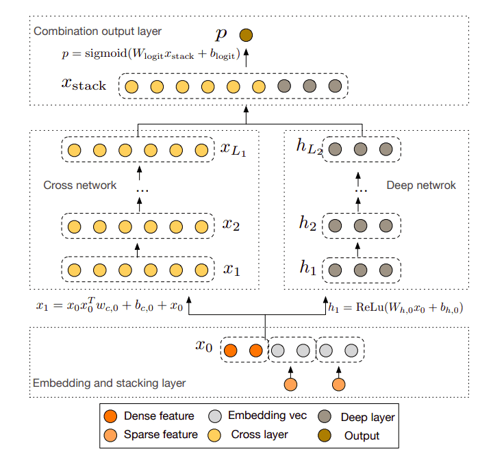DCN. Source: Deep & Cross Network for Ad Click Predictions

The cross-network takes advantage of a very powerful idea: it applies feature crossing at each layer. As the layer depth increases, the degrees of feature crossing increase as well. The original paper provides an intuitive image of how the cross-layer works:

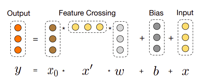A cross layer. Source: Deep & Cross Network for Ad Click Predictions

In the image, the input $x$ is interacting with the original input $x_0$ producing higher-order cross features. The input $x$ is also added back to the output in a type of residual connection. Therefore, the output $y$ is a higher-order feature that is passed to the next layer.

The Deep network, on the other hand, is a traditional multilayer perceptron. The combination of the two networks gives us the final prediction.

The authors present DCN as an extension of factorization machines. The FM is limited in representing cross-terms of degree 2. DCN, in contrast, is able to construct cross-terms of a higher degree $|a|$ . $|a|$ is bounded by the number of layers.

DLRM

Deep Learning Recommendation Model (DLRM) was initially proposed by Facebook. It originates from two different perspectives: recommendation systems and predictive analytics. Predictive analytics rely on statistical models to predict the probability of events based on the given data. In conjunction with traditional recommendation strategies, we can build highly personalized recommendations.

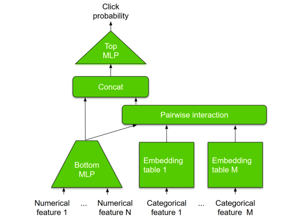DLRM. Source: Optimizing the Deep Learning Recommendation Model on NVIDIA GPUs

Numerical and Dense features are processed through a Multi-Layer Perceptron (MLP). Categorical and sparse features are modeled through embedding tables. The interaction between all features is computed by taking the dot-product between all pairs, following the principles of factorization machines.

The dot-products are then concatenated with the original processed dense features and then transformed into a final probability using another MLP.

It is worth mentioning that the authors did a great job on parallelizing and optimizing the model. I won’t go into many details here because it exceeds the purpose of this article but feel free to advise the original paper.

Graph Neural Networks for Recommendations

As a final mention, I couldn’t avoid a reference on Graph Neural Networks (GNNs) for recommendation systems.

Intuition: the available data and features might be better represented in a graph structure.

Graph neural networks can be used to model feature interactions and generate high-quality embeddings for all users and items.

GNNs can be used for different types of recommendations. General recommendations disregard the notion of time and deals only with user-item interactions and contextual information. Sequential recommendation, on the other hand, seeks to capture transitional patterns in the user’s behavior.

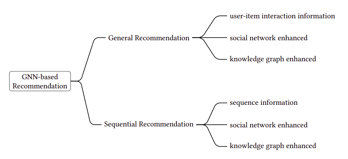Graph Neural Networks in Recommender Systems: A Survey

If you want to dive deeper into GNN-based systems, here is a recent survey that contains everything you need: Graph Neural Networks in Recommender Systems: A Survey

State of art implementations include: IGMC, MG-GAT, DANSER and DGRec

Conclusion

Deep Learning opened a new chapter in recommendation systems and helped accelerate the field by rapid steps. From 2009 where the infamous 1 million Netflix prize competition took place until today, recommenders have evolved tremendously. Most strategies are based on a combination of low-level and high-level representation, which have been proven to work very well. Sequence-based techniques, graph neural networks, and even reinforcement learning methods (which we didn’t mention) can be excellent alternatives in specific problems.

If you want to play around with the different methods, TensorFlow Recommenders is a great package to get you started. As a side material, the Recommender Systems Specialization by the University of Michigan is an excellent choice. Feel free to ping us on social for any questions, corrections, or suggestions.

That’s all folks.

References

[1] He, Xiangnan, et al. “Neural Collaborative Filtering.” ArXiv:1708.05031 [Cs], Aug. 2017.
[2] Cheng, Heng-Tze, et al. “Wide & Deep Learning for Recommender Systems.” ArXiv:1606.07792 [Cs, Stat], June 2016.
[3] “Wide & Deep Learning: Better Together with TensorFlow.” Google AI Blog.
[4] Guo, Huifeng, et al. “DeepFM: A Factorization-Machine Based Neural Network for CTR Prediction.” ArXiv:1703.04247 [Cs], Mar. 2017.
[5] Steffen Rendle, Factorization Machines, ICDM 2010, The 10th IEEE International Conference on Data Mining, Sydney, Australia, 14-17 December 2010
[6] Sedhain, Suvash, et al. “AutoRec: Autoencoders Meet Collaborative Filtering.” Proceedings of the 24th International Conference on World Wide Web, Association for Computing Machinery, 2015, pp. 111–12. ACM Digital Library, doi:10.1145/2740908.2742726.
[7] Quadrana, Massimo, et al. “Sequence-Aware Recommender Systems.” ArXiv:1802.08452 [Cs], Feb. 2018.
[8] Wang, Ruoxi, et al. “Deep & Cross Network for Ad Click Predictions.” ArXiv:1708.05123 [Cs, Stat], Aug. 2017.
[9] Naumov, Maxim, et al. “Deep Learning Recommendation Model for Personalization and Recommendation Systems.” ArXiv:1906.00091 [Cs], May 2019.
[10] Wu, Shiwen, et al. “Graph Neural Networks in Recommender Systems: A Survey.” ArXiv:2011.02260 [Cs], Apr. 2021.
[11] "Overview of recommender systems — dive into deep learning 0.16.4 documentation"
[12] Le, James. “Recommendation System Series Part 1: An Executive Guide to Building Recommendation System.” Medium, 28 June 2020,
[13] Koren, Yehuda, et al. “Matrix Factorization Techniques for Recommender Systems.” Computer, vol. 42, no. 8, Aug. 2009, pp. 30–37. IEEE Xplore, doi:10.1109/MC.2009.263.
[14] Zhang, Shuai, et al. “Deep Learning Based Recommender System: A Survey and New Perspectives.” ACM Computing Surveys, vol. 52, no. 1, Feb. 2019, pp. 1–38.,doi:10.1145/3285029.
[15] Marcel Kurovski, 47th #ebaytechtalk: Deep Learning for recommender systems
[16] Nick Pentreath, Deep learning for recommender systems

* Disclosure: Please note that some of the links above might be affiliate links, and at no additional cost to you, we will earn a commission if you decide to make a purchase after clicking through.