How Graph Neural Networks (GNN) work: introduction to graph convolutions from scratch

In this tutorial, we will explore graph neural networks and graph convolutions. Graphs are a super general representation of data with intrinsic structure. I will make clear some fuzzy concepts for beginners in this field.

The most intuitive transition to graphs is by starting from images.

Why?

Because images are highly structured data. Their components (pixels) are arranged in a meaningful way. If you change the way pixels are structured the image loses its meaning. Additionally, images have a very strong notion of locality.

Image by Author. Location: Evia, Greece

As you can see, the pixels are arranged in a grid, which is the structure of the image. Since structure matters, it makes sense to design filters to group representation from a neighborhood of pixels, that is convolutions!

The pixels also have one (grayscale) or more intensity channels. In a general form, each pixel has a vector of features that describe it. Thus, the channel intensities could be regarded as the signal of the image.

The reason that we don’t think of images in a pre-described way is that the representation of structure and signal (features) are merged together.

The key concept to understand graphs is the decomposition of structure and signal (features), which make them so powerful and general methods.

Code: The article is accompanied by a colab notebook.

Decomposing features (signal) and structure

As we saw in Transformers, natural language can also be decomposed to signal and structure. The structure is the order of words, which implies syntax and grammar context. Here is an illustrative example:

Image by Author

The features will now be a set of word embeddings and the order will be encoded in the positional embeddings.

Graphs are not any different: they are data with decomposed structure and signal information.

Real-world signals that we can model with graphs

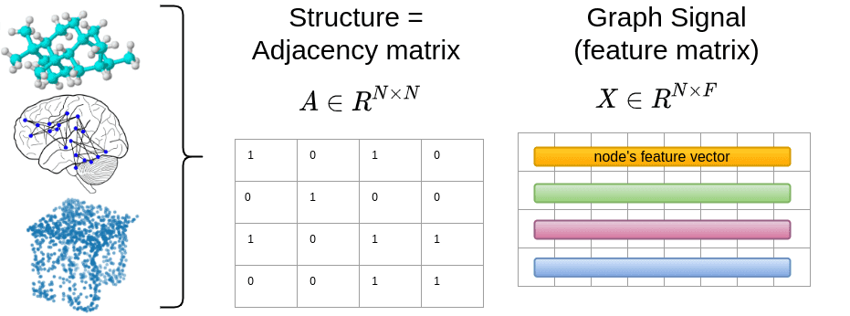
As long as you can define these two representations, you can model anything you want with graphs. Formally, the words or pixels are simply nodes, denoted by $N$. The connectivity/structure will be defined by a $N \times N$ matrix, the so-called Adjacency matrix $A$. The element $i,j$ of $A$ will tell us if node $i$ is connected to node $j$.

The signal for each node will be $X \in R^{N \times F}$. $F$ is the number of features. For example, an RGB image has $F=3$ features, while for a word will be the embedding dimension.

To this end, we can represent brain graphs from functional medical imaging, social networks, point clouds, and even molecules and proteins.

Image by Author

In the image above, the connectivity is shown to be binary, which is the most common form but it can be non-binary also.

For the record, a point cloud is just a set of data points in space. The points may represent a 3D object, like the desk that we just saw.

Note that the diagonal of $A$ is shown to contain ones, which is usually the case in graph neural networks for training stability reasons, although in the general case it has zeros, indicating no-self connections.

Having that set, it’s time to make sense out of some maths.

The basic maths for processing graph-structured data

We already defined the graph signal $X \in R^{N \times F}$ and the adjacency matrix $A \in N \times N$. A very important and practical feature is the degree of each node, which is simply the number of nodes that it is connected to. For instance, every non-corner pixel in an image has a degree of 8, which is the surrounding pixels.

If $A$ is binary the degree corresponds to the number of neighbors in the graph. In general, we calculate the degree vector by summing the rows of $A$. Since the degree corresponds to some kind of feature that is linked to the node, it is more convenient to place the degree vector in a diagonal $N \times N$ matrix :

import torch
# rand binary Adj matrix
a = torch.rand(3,3)
a[a>0.5] = 1
a[a<=0.5] = 0
def calc_degree_matrix(a):
 return torch.diag(a.sum(dim=-1))
d = calc_degree_matrix(a)

Results in:

A =   ([[0., 1., 1.],
        [1., 1., 0.],
        [0., 1., 0.]])

D =   ([[2., 0., 0.],
        [0., 2., 0.],
        [0., 0., 1.]])

The degree matrix $D$ is fundamental in graph theory because it provides a single value of each node. It is also used for the computation of the most important graph operator: the graph laplacian!

The graph Laplacian

The graph Laplacian is defined as:

In fact, the diagonal elements of $L$ will have the degree of the node, if $A$ has no self-loops. On the other hand, the non-diagonal elements $L_{ij} = -1 , when \quad i \neq j$ if there is a connection. If there is no connection $L_{ij} = 0 , when \quad i \neq j$

In practice:

def create_graph_lapl(a):
 return calc_degree_matrix(a)-a

print(a)
print(create_graph_lapl(a))

Results in:

A =   ([[1., 1., 1., 1., 0.],
        [1., 1., 0., 1., 0.],
        [0., 0., 0., 1., 1.],
        [0., 0., 0., 1., 1.],
        [1., 1., 1., 1., 0.]])

L =   ([[ 3., -1., -1., -1.,  0.],
        [-1.,  2.,  0., -1.,  0.],
        [ 0.,  0.,  2., -1., -1.],
        [ 0.,  0.,  0.,  1., -1.],
        [-1., -1., -1., -1.,  4.]])

However, in graph neural networks we use its normalized version. Why?

Because nodes have varying connectivity and as a result a big range of degree values on $D$. For example, in a graph with 100 nodes one node may have only one connection and another 100 connections.

This will create huge problems when processing with gradient-based methods, as we have discussed in the normalization article.

You may be wondering what we gain with this fancy math. It’s better to see it with your own eyes:

def calc_degree_matrix_norm(a):
 return torch.diag(torch.pow(a.sum(dim=-1),-0.5))

def create_graph_lapl_norm(a):
 size = a.shape[-1]
 D_norm = calc_degree_matrix_norm(a)
 L_norm = torch.ones(size) - (D_norm @ a @ D_norm )
 return L_norm

Output:

A =     ([[0., 0., 1., 1., 1.],
          [1., 0., 1., 0., 1.],
          [1., 0., 0., 0., 1.],
          [0., 1., 0., 0., 0.],
          [0., 0., 1., 1., 0.]])

L_norm = ([[1.0000, 1.0000, 0.5918, 0.4226, 0.5918],
          [0.6667, 1.0000, 0.5918, 1.0000, 0.5918],
          [0.5918, 1.0000, 1.0000, 1.0000, 0.5000],
          [1.0000, 0.4226, 1.0000, 1.0000, 1.0000],
          [1.0000, 1.0000, 0.5000, 0.2929, 1.0000]])

Actually, we are no longer dependent on the varying number of degrees that can lead to instabilities. Now all the diagonal elements will be ones when there is at least one connection of the graph’s node independent of the node’s degree. The node’s degree will now influence the non-diagonal elements which will be $\frac{1}{(deg(n_i) deg(n_j) )^{1/2} }$.

In graph neural networks a slightly alternated version is often used:

Where $I$ denotes the identity matrix, which adds self-connections. From now on, we will refer to this as a normalized graph laplacian.

With this trick, the input can be fed into a gradient-based algorithm without causing instabilities.

Before we move one, it is crucial to see some properties of the graph Laplacian.

Laplacian eigenvalues and eigenvectors

Eigenvalues and eigenvectors are the heart of a matrix. I like to think of them as frequencies.

Insight: The zeroth eigenvalue indicates whether the graph is connected or not.

In particular, if a graph has $k$ connected components, then eigenvalue 0 has multiplicity k (i.e. k distinct non-trivial eigenvectors).

The multiplicity of the zero eigenvalue of the graph Laplacian is equal to the number of connected components.

The following graph would have 2 zero eigenvalues since it has 2 connected components:

Image by Author

As you can see there is no connection between the nodes on the sub-graphs. If you start from any node, you cannot traverse all the nodes.

In the most common case, a graph that has a single zero eigenvalue is connected, meaning that starting from any node you can visit all the other nodes with some steps, like in the following example:

import matplotlib.pyplot as plt
import networkx as nx
G = nx.petersen_graph()
plt.subplot(121)
nx.draw(G, with_labels=False, font_weight='bold')
plt.subplot(122)
nx.draw_shell(G, nlist=[range(5, 10), range(5)], with_labels=False, font_weight='bold')

options = {
   'node_color': 'blue',
   'node_size': 100,
   'width': 2,
}
plt.subplot(221)
nx.draw_random(G, **options)
plt.subplot(222)
nx.draw_circular(G, **options)
plt.subplot(223)
nx.draw_spectral(G, **options)
plt.subplot(224)
nx.draw_shell(G, nlist=[range(5,10), range(5)], **options)

Outputs the following graphs:

Spectral image segmentation with graph laplacian

In graphs, the smallest non-zero eigenvalue has been used for “spectral” image segmentation from the 90s. By converting a grayscale image to a graph (see code below), you can divide an image based on its slowest non-zero frequencies/eigenvalues.

Spectral segmentation is an unsupervised algorithm to segment an image based on the eigenvalues of the laplacian.

In the following example, we divide an image into 3 segments (clusters):

import numpy as np
from scipy import misc
from skimage.transform import resize
import matplotlib.pyplot as plt
from numpy import linalg as LA
from scipy.sparse import csgraph
from sklearn.feature_extraction.image import img_to_graph
from sklearn.cluster import spectral_clustering


re_size = 64 # downsampling of resized rectangular image
img = misc.face(gray=True)  # retrieve a grayscale image
img = resize(img, (re_size, re_size))
mask = img.astype(bool)
graph = img_to_graph(img, mask=mask)
# Take a decreasing function of the gradient: we take it weakly
# dependant from the gradient the segmentation is close to a voronoi
graph.data = np.exp(-graph.data / graph.data.std())
labels = spectral_clustering(graph, n_clusters=3)
label_im = -np.ones(mask.shape)
label_im[mask] = labels

plt.figure(figsize=(6, 3))
plt.imshow(img, cmap='gray', interpolation='nearest')

plt.figure(figsize=(6, 3))
plt.imshow(label_im, cmap=plt.cm.nipy_spectral, interpolation='nearest')
plt.show()

Note that this method does not scale so well since $N$ pixels would require a $N \times N$ Adjacency matrix.

For more information on eigenvalues and eigenvectors, check out 3B1B’s video:

How to represent a graph: types of graphs

Directed VS Undirected graphs

Graphs can have direction too. This particularity is injected into the adjacency matrix. Specifically a symmetric $A$ refers to an undirected graph. On the other hand, directed graphs have a non-symmetric $A$.

There is also the notion of traversing a graph in terms of steps, called hops. As an example, in the undirected graph to go from node 5 to node 1, you'll need 2 hops.

Weighted VS unweighted graphs

Graphs can also have weighted connections. The adjacency matrix is not always binary. You can model your data in a more flexible way.

For example, in point clouds, the 3D Euclidean distance between 2 points may be encoded in a weighted adjacency matrix. Another example may be the distance between cities on the earth that can be encoded with the spherical distance.

Here is an illustration of a weighted undirected graph.

By now, I think you get the idea that graphs are extremely general representations.

The COO format

It is very common to store the adjacency matrix in the Coordinate Format (COO) format: we index the row and column of $A$ and optionally we can also associate a value (data). Here is an example using the scipy library:

import numpy as np
import scipy.sparse as sparse
row =  np.array([0, 3, 1, 0])
col =   np.array([0, 3, 1, 2])
data = np.array([4, 5, 7, 9])

mtx = sparse.coo_matrix((data, (row, col)), shape=(4, 4))
mtx.todense()

Outputs:

matrix([[4, 0, 9, 0],
        [0, 7, 0, 0],
        [0, 0, 0, 0],
        [0, 0, 0, 5]])

I am highlighting the representation here because it might be confusing for beginners in the field. It is equivalent to storing the whole $A$ matrix. It is just more efficient for sparse graph data.

Types of graph tasks: graph and node classification

We discussed a bit about the input representation. But what about the target output? The most basic tasks in graph neural networks are:

• Graph classification: We have a lot of graphs and we would like to find a single label for each individual graph (similar to image classification). This task is casted as a standard supervised problem. In graphs, you will see the term Inductive learning for this task.

• Node classification: Usually in this type of task we have a huge graph (>5000 nodes) and we try to find a label for the nodes (similar to image segmentation). Importantly, we have very few labeled nodes to train the model (for instance <5%). The aim is to predict the missing labels for all the other nodes in the graph. That’s why this task is formulated as a semi-supervised learning task or Transductive learning equivalently. It’s called semi-supervised because even though the nodes do not have labels, we feed the graph (with all the nodes) in the neural network and formulate a supervised loss term for the labeled nodes only.

Source: Ground AI

Next, I will provide some minimal theory on how we process graph data.

How graph convolutions layer are formed

Principle: Convolution in the vertex domain is equivalent to multiplication in the graph spectral domain.

The most straightforward implementation of a graph neural network would be something like this:

Where $W$ is a trainable parameter and $Y$ the output.

Why? Because now we have to account not just for the signal $X$ but also for the structure/connectivity ($A$).

The thing is that A is usually binary and has no interpretation.

By definition, multiplying a graph operator by a graph signal will compute a weighted sum of each node’s neighborhood. And it’s amazing that this can be expressed with a simple matrix multiplication!

Instead of A, we would like to have a more expressive operator. In general, when you multiply a graph operator by a graph signal, you get a transformed graph signal.

That’s why we use the normalized Laplacian instead of $A$. Furthermore, the graph Laplacian L has a direct interpretation. When raised to the power $K$, it traverses nodes that are up to $p$ steps away, thus introducing the notion of locality.

Formally, by multiplying the signal with a Laplacian power K, $L^K$ can be interpreted as expressing the graph constructed from the $K$-hops thus providing the desired localization property (similar to convolutions).

In the simplest case we have the GCN layer:

Notice that I used a slightly modified version of the Laplacian, which helps encounter training instabilities by adding self-loops. Self-loops are added by adding the identity matrix to the adjacency matrix while recomputing the degree matrix.

In this case, each layer will consider only its direct neighbors since we use the first power of laplacian $L^1$. This is similar to a 3x3 kernel in classical image convolution, wherein we aggregate information from the direct pixel’s neighborhood.

But we may extend this idea. Actually, the originally proposed graph convolution used and defined higher powers of the graph Laplacian.

The background theory of spectral graph convolutional networks

Feel free to skip this section if you don’t really care about the underlying math. I leave it here for self-completeness.

In fact, the initial method proposed to use the powers of Laplacian to increase the K-hops in each layer. As it is described in Defferrard et al on “Convolutional neural networks on graphs with fast localized spectral filtering”, the convolution of graph signal $X$ can be defined in the “spectral” domain.

Spectral basically means that we will utilize the Laplacian eigenvectors. Therefore convolution in graphs can be approximated by applying a filter $g$ in the eigenvalues of the Laplacian.

where $\mathbf{U}$ represents the eigenvectors of $\mathbf{L}$ and $\mathbf{\Lambda}$ is a diagonal matrix whose elements are the corresponding eigenvalues.

The recurrent Chebyshev expansion

However, the computation of the eigenvalues would require a Singular Value Decomposition (SVD) of $\mathbf{L}$, which is computationally costly. Therefore, we will approximate this operation with the so-called Chebyshev expansion.

This is similar to approximating a function with a Taylor series based on its derivatives: basically, we compute a sum of its derivatives at a single point. The Chebyshev approximation is a recurrent expansion that uses a matrix (here $\mathbf{L}$) to estimate the matrix in any given power $K$, thus avoiding the $K$ square matrix multiplications.

The bigger the power the bigger the local receptive field of our graph neural network layer.

To this end, we will design a filter $g$ parametrized as a polynomial function of L, which can be calculated from a recurrent Chebyshev expansion of order K.

We will work with a rescaled graph laplacian to avoid the SVD.

The big picture of the graph convolutional layer will be:

Moreover, instead of doing $K$ multiplications of $L_{norm}$ to calculate the $K$-th power in the spectral filtering, we will use the Chebyshev expansion in the laplacian:

The index $p$ indicates the power. In particular, each graph conv. layer will do the following:

with $\theta_{v}= [\theta_0, \theta_1, .. , \theta_{K-1} ]$ are the learnable coefficients.

The first two recurrent terms of the polynomial expansion are calculated as: $\tilde{\mathbf{X}}_{0} = \mathbf{X}$ and $\tilde{\mathbf{X}}_{1} = \tilde{\mathbf{L}}_{h} \mathbf{X}$.

Thus, the graph signal $\mathbf{X}$ is projected onto the Chebyshev basis (powers) $\mathbf{T}_p( \tilde{\mathbf{L}}_{h})$ and concatenated (or summed) for all orders $p \in [0,K-1]$.

You can imagine the projection onto multiple powers of laplacian as an inception module in CNNs. As a result, multiple complex relationships between neighboring vertices are gradually captured in each layer. The receptive field is controlled by $K$ and the trainable parameters $\theta_{v}$ adjust the contribution of each Chebyshev basis.

What we actually do under the hood: spectral filtering on the eigenvalues

Even though I will provide an implementation of the pre-described method, we are actually raising the eigenvalues to the power K.

If you look at the matrix properties the power of the Laplacian is applied in the eigenvalues:

So even though we use the laplacian directly we are actually operating on the eigenvalues:

with $\mathbf{T}_p( \tilde{\mathbf{\Lambda}})= 2 \tilde{\mathbf{\Lambda}} \mathbf{T}_{p-1}( \tilde{\mathbf{\Lambda}}) - \mathbf{T}_{p-2}( \tilde{\mathbf{\Lambda}})$, $\tilde{\mathbf{\Lambda}}= \frac{2}{\lambda_{max}} \mathbf{\Lambda}-\mathbf{I}$ and $\theta\in \mathbb{R}^K$ is the vector of the spectral coefficients.

Insight: By approximating a higher power $K$ of the Laplacian, we actually design spectral filters that enable each layer to aggregate information from $K$-hops away neighbors in the graph, similarly to increasing the kernel size of a convolutional kernel.

Illustration of the general graph convolution method

Here is a rough implementation of how this works in practice:

import torch
import torch.nn as nn

def find_eigmax(L):
   with torch.no_grad():
       e1, _ = torch.eig(L, eigenvectors=False)
       return torch.max(e1[:, 0]).item()

def chebyshev_Lapl(X, Lapl, thetas, order):
 list_powers = []
 nodes = Lapl.shape[0]

 T0 = X.float()

 eigmax = find_eigmax(Lapl)
 L_rescaled = (2 * Lapl / eigmax) - torch.eye(nodes)

 y = T0 * thetas[0]
 list_powers.append(y)
 T1 = torch.matmul(L_rescaled, T0)
 list_powers.append(T1 * thetas[1])

 # Computation of: T_k = 2*L_rescaled*T_k-1  -  T_k-2
 for k in range(2, order):
     T2 = 2 * torch.matmul(L_rescaled, T1) - T0
     list_powers.append((T2 * thetas[k]))
     T0, T1 = T1, T2
 y_out = torch.stack(list_powers, dim=-1)
 # the powers may be summed or concatenated. i use concatenation here
 y_out = y_out.view(nodes, -1) # -1 = order* features_of_signal
 return y_out

features = 3
out_features = 50
a = create_adj(10)
L = create_graph_lapl_norm(a)
x = torch.rand(10, features)
power_order = 4 # p-hops
thetas = nn.Parameter(torch.rand(4))

out = chebyshev_Lapl(x,L,thetas,power_order)

print('cheb approx out powers concatenated:', out.shape)
# because we used concatenation  of the powers
# the out features will be power_order * features
linear = nn.Linear(4*3, out_features)

layer_out = linear(out)
print('Layers output:', layer_out.shape)

Outputs:

cheb approx out powers concatenated: torch.Size([10, 12])
Layers output: torch.Size([10, 50])

It would be interesting to train this implementation, but now I just presented it for educational purposes. We will instead train the simplest form which will lead us to a 1-hop away GCN layer.

Implementing a 1-hop GCN layer in Pytorch

For this tutorial, we will train a simple 1-hop GCN layer in a small graph dataset. Our GCN layer will be defined by the following equations:

Here is what this layer looks like in Pytorch:

import numpy as np
import torch
from torch import nn
import torch.nn.functional as F

def device_as(x,y):
  return x.to(y.device)

# tensor operations now support batched inputs
def calc_degree_matrix_norm(a):
  return torch.diag_embed(torch.pow(a.sum(dim=-1),-0.5))

def create_graph_lapl_norm(a):
  size = a.shape[-1]
  a +=  device_as(torch.eye(size),a)
  D_norm = calc_degree_matrix_norm(a)
  L_norm = torch.bmm( torch.bmm(D_norm, a) , D_norm )
  return L_norm

class GCN_AISUMMER(nn.Module):
    """
    A simple GCN layer, similar to https://arxiv.org/abs/1609.02907
    """
    def __init__(self, in_features, out_features, bias=True):
    super().__init__()
    self.linear = nn.Linear(in_features, out_features, bias=bias)

    def forward(self, X, A):
        """
        A: adjecency matrix
        X: graph signal
        """
        L = create_graph_lapl_norm(A)
        x = self.linear(X)
        return torch.bmm(L, x)

Training our GCN for graph classification

I will now use the open-source graph data from the University of Dortmund. We will use the MUTAG dataset because it is small and can be trained on google colab. Each node contains a label from 0 to 6 which will be used as a one-hot-encoding feature vector. From the 188 graphs nodes, we will use 150 for training and the rest for validation. Finally, we have two classes.

The goal is to demonstrate that graph neural networks are a great fit for such data. You can find the data-loading part as well as the training loop code in the notebook. I chose to omit them for clarity. I will instead show you the result in terms of accuracy.

Here is the total graph neural network architecture that we will use:

import torch
from torch import nn
import torch.nn.functional as F

class GNN(nn.Module):
  def __init__(self,
                    in_features = 7,
                    hidden_dim = 64,
                    classes = 2,
                    dropout = 0.5):
    super(GNN, self).__init__()

    self.conv1 = GCN_AISUMMER(in_features, hidden_dim)
    self.conv2 = GCN_AISUMMER(hidden_dim, hidden_dim)
    self.conv3 = GCN_AISUMMER(hidden_dim, hidden_dim)
    self.fc = nn.Linear(hidden_dim, classes)
    self.dropout = dropout

  def forward(self, x,A):
    x = self.conv1(x, A)
    x = F.relu(x)
    x = self.conv2(x, A)
    x = F.relu(x)
    x = self.conv3(x, A)
    x = F.dropout(x, p=self.dropout, training=self.training)
    # aggregate node embeddings
    x = x.mean(dim=1)
    # final classification layer
    return self.fc(x)

Insight: It may sound counter-intuitive and obscure but the adjacency matrix is used in all the graph conv layers of the architecture. This gives graph neural networks a strong inductive bias to respect the initial graph structure in all their layers.

Here is the results of training:

Epoch: 010, Train Acc: 0.6600, Val Acc: 0.6842 || Best Val Score: 0.6842 (Epoch 001)
Epoch: 020, Train Acc: 0.6600, Val Acc: 0.6842 || Best Val Score: 0.6842 (Epoch 001)
Epoch: 030, Train Acc: 0.6800, Val Acc: 0.7105 || Best Val Score: 0.7895 (Epoch 027)
Epoch: 040, Train Acc: 0.7467, Val Acc: 0.6579 || Best Val Score: 0.7895 (Epoch 027)
Epoch: 050, Train Acc: 0.7400, Val Acc: 0.6579 || Best Val Score: 0.7895 (Epoch 027)
Epoch: 060, Train Acc: 0.7200, Val Acc: 0.6842 || Best Val Score: 0.7895 (Epoch 027)
Epoch: 070, Train Acc: 0.7667, Val Acc: 0.7105 || Best Val Score: 0.7895 (Epoch 027)
Epoch: 080, Train Acc: 0.7600, Val Acc: 0.7105 || Best Val Score: 0.7895 (Epoch 027)
Epoch: 090, Train Acc: 0.7600, Val Acc: 0.7105 || Best Val Score: 0.7895 (Epoch 027)
Epoch: 100, Train Acc: 0.7533, Val Acc: 0.6842 || Best Val Score: 0.7895 (Epoch 027)
Epoch: 110, Train Acc: 0.7533, Val Acc: 0.6842 || Best Val Score: 0.7895 (Epoch 027)
Epoch: 120, Train Acc: 0.7800, Val Acc: 0.7895 || Best Val Score: 0.7895 (Epoch 027)
Epoch: 130, Train Acc: 0.7800, Val Acc: 0.7368 || Best Val Score: 0.7895 (Epoch 027)
Epoch: 140, Train Acc: 0.7600, Val Acc: 0.6316 || Best Val Score: 0.7895 (Epoch 027)
Epoch: 150, Train Acc: 0.7400, Val Acc: 0.6579 || Best Val Score: 0.7895 (Epoch 027)
Epoch: 160, Train Acc: 0.7733, Val Acc: 0.7105 || Best Val Score: 0.8158 (Epoch 157)
Epoch: 170, Train Acc: 0.7867, Val Acc: 0.7632 || Best Val Score: 0.8158 (Epoch 157)
Epoch: 180, Train Acc: 0.7867, Val Acc: 0.7368 || Best Val Score: 0.8158 (Epoch 157)
Epoch: 190, Train Acc: 0.7800, Val Acc: 0.7105 || Best Val Score: 0.8158 (Epoch 157)
Epoch: 200, Train Acc: 0.7533, Val Acc: 0.6579 || Best Val Score: 0.8158 (Epoch 157)
Epoch: 210, Train Acc: 0.7733, Val Acc: 0.6842 || Best Val Score: 0.8158 (Epoch 157)
Epoch: 220, Train Acc: 0.7600, Val Acc: 0.6842 || Best Val Score: 0.8158 (Epoch 157)
Epoch: 230, Train Acc: 0.7867, Val Acc: 0.7105 || Best Val Score: 0.8158 (Epoch 157)
Epoch: 240, Train Acc: 0.7733, Val Acc: 0.7105 || Best Val Score: 0.8158 (Epoch 157)

Note that I didn’t play so much on the hyperparameters. Feel free to propose your hyperparameter and other improvements. For the record, the state-of-the-art on this dataset is more than 90% with a 10-cross validation method.

Practical issues when dealing with graphs

One of the practical problems with graph data is the varying number of nodes that makes batching graph data difficult. The solution?

Block-diagonal matrices:

Source: Pytorch Geometric

This matrix operation actually gives us a bigger graph with batch size (2 here) non-connected components (subgraphs). I will let you guess what will happen to the eigenvalues.

Since I purposely avoided this part in the tutorial I used a batch size of 1 :).

Another issue, especially for graph classification is how to produce a single label when you have the node embeddings. By node embeddings I mean the transformed learned feature representation for each node (X1’ and X2’ in the figure above). This is called the readout layer in the graph literature. Basically, we will aggregate the node representations. Of course, there exists a lot of “readout” layers, but the most common is to use a mean or max operation on the node embeddings.

Other misleading experimental results may be the instability in training compared with classical CNN in images that produce super smooth curves. Don’t worry, it's extremely rare that you will get a textbook’s training curve! And it’s completely fine!

Conclusion

This tutorial was a deep intro to graphs for those that had no experience with these kinds of data. I provided a lot of perspectives to make the concepts clear and intuitive. I also provided code to better illustrate my points.

If you are serious about going deeper into the graph neural network area, I would suggest learning to work with Pytorch Geometric. You will need a GPU to play with it but there are a lot of tutorials and a lot of recent graph-based models. I would like to recommend an awesome video by Petar Veličković on Theoretical Foundations of Graph Neural Networks:

If you learned something new, the best way to help spread accessible AI content is to share our article on social media.

Deep Learning in Production Book 📖

Learn how to build, train, deploy, scale and maintain deep learning models. Understand ML infrastructure and MLOps using hands-on examples.

Learn more

* Disclosure: Please note that some of the links above might be affiliate links, and at no additional cost to you, we will earn a commission if you decide to make a purchase after clicking through.