
Sometimes you think you understand something, but you fail to explain it. This is the time that you have to look back from a different perspective and start over. When you dig in medical images you will see different concepts to seem vague and non-intuitive, at least in the beginning. You will see people discussing DICOM and coordinate systems you have never heard before. As a result, a lot of misconceptions and confusions are born. If you are in this position, or if you would like to know about AI in medical imaging this article is for you.
Back in 2017, when I applied for my master’s degree in biomedical engineering everybody asked me why, as I was already obsessed with deep learning. Now, every multidisciplinary deep learning research project requires domain knowledge such as medical imaging. Interestingly, the funding in the AI Healthcare domain is continuously increasing. As an quantitative example of first google search that one can find out:
The market for machine learning in diagnostic imaging will top 2 billion $ by 2023.
So, the reason that I decided to write this article is to help ML people dive into medical imaging.
In a previous article, I talked about a common deep learning pipeline applied to multi-modal magnetic resonance datasets. All of that of course with our under development open source pytorch library called medicalzoo-pytorch. However, I didn't dive into the particularities of the medical world too much. In the end, I used already processed data from an ML competition (and not from a messy hospital), so somebody else did the dirty work for me. This tutorial is partly based in the nipy [1] and 3D Slicer.org [2] documentations for medical images and Dicom files.
To dive deeper into how AI is used in Medicine, you can’t go wrong with the AI for Medicine online course, offered by Coursera. If you want to focus on medical image analysis with deep learning, I highly recommend starting from the Pytorch-based Udemy Course.
However, I decided to adapt and revisit the concepts and make them more familiar to Machine and deep learning engineers. There are a lot of assumptions that ML engineers have no idea about. Other multi-disciplinary projects have this kind of terminology problem. To this end, I considered it of great value to bridge this gap between medical imaging concepts and deep learning that no one talks about, in this humble post. At least, I'll try my best, one concept at a time!
Notation: medical image tutorials often call the MRI and CT exams as ‘model’. For convenience, and to avoid misconceptions we will use the world modality, throughout this tutorial to refer to any kind of medical image exam. The word ‘view’ and ‘plane’ are used interchangeably.
We are all set to go into the medical imaging world!
The coordinate systems in medical imaging
A coordinate system is a method for identifying the location of a point. In the medical world, there are three coordinate systems commonly used in imaging applications: the world, anatomical, and the medical image coordinate system.
 Source: 3D slicer documentation [2]
World coordinate system
The world coordinate system is a Cartesian coordinate system in which a medical image modality (e.g. an MRI scanner or CT) is positioned. Every medical modality has its own coordinate system, but there is only one world coordinate system to define the position and orientation of each modality.
Anatomical coordinate system
The most important model coordinate system for medical imaging techniques is the anatomical space (also called the patient coordinate system). This space consists of three planes to describe the standard anatomical position of a human:
the axial plane
the sagittal plane
the coronal plane
It is worth mentioning that this system was invented for better communication between doctors and radiologists.
Tip: In order to understand the anatomical planes, you have to visualize a standing human looking at you.
Moreover, in this system everything is relevant. Thus, the 3D position is defined along the anatomical axes of anterior-posterior (front-back) and left-right and inferior-superior, as we will see. By this sense, all axes have their notation in a positive direction.
Axial plane
The axial plane is actually when you place your point of view above the patient and look down. Depending on the region of the 3D medical image you will observe different anatomical structures. For a 3D total body scan, if you had a control-bar over this 2D view you would start from a 2D slice of the head, and by increasing you would end up in the legs. Let’s practically call this view the “drone plane” or “top-view”. Below you can see different slices of a brain MRI.
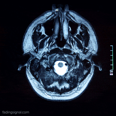
For anatomical consistency reasons, a slice near the head is referred to as superior compared to a slice closer to the feet, which is called inferior.
Does it seem complex? It is, I know! But it's important for your mental sanity if you want to survive in the field. Unfortunately, the other two planes assume different directions for positive 😢.
For completeness, and to present something a little bit more recent below you see an axial CT of a patient. Radiologists have highlighted irregularities that may be due to COVID. I am just resharing the image here to illustrate the axial slice, looking from the top to the patient. The particular slice refers in the lungs.

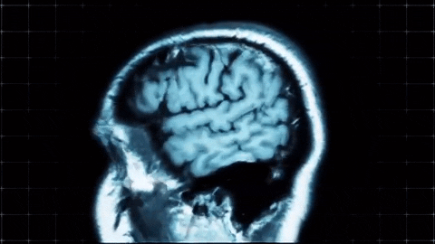
Sagittal plane
Basically, this is a side view. Instead of looking from above the patient, now we look from the side. The side can be either right or left. Which side and direction is the positive one, depends on the coordinate system! The sure thing is that from this view (plane) you can see the patient's ear! As you move through this axis you see the projected tissues like lungs, bones.
A sagittal view of a brain MRI can be illustrated below:
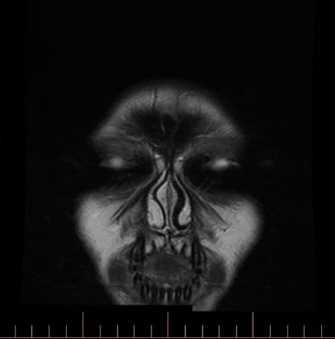
Coronal plane
In this view, we traverse either by looking in the eyes (anterior plane) or by looking in the back of a patient (posterior plane). I hope you get the idea by now.
In order to make sure that you will never forget what a coronal plane is, I found this awful halloween gif:
The highlighted terms in bold define the different Anatomical coordinate systems, as illustrated below.
Tip: LPS is used by DICOM images and by the ITK toolkit (simpleITK in python), while 3D Slicer and other medical software use RAS.
Medical Image coordinate system (Voxel space)
This is the part that comes more intuitively for people with a computer vision background. If you have any experience with other 3D deep learning domains, I can assure you that this is the place that you will find some rationality and relevant context, at last!
Medical modalities create 3D arrays/tensors of points and cells which start at the upper left corner, similar to an RGB camera for 2D. The i axis increases to the right (width), the j axis to the bottom (height), and the k axis backward (the 3rd similarly to the feature maps of a conv net).
In addition to the intensity value of each voxel (i j k), the origin (i.e. MRI) and spacing of the coordinates are stored in the meta-data of the medical image (either dicom tags, header file of nifty images, you name it.. ).
Voxel spacing is basically the real size of the voxel that corresponds to a 3D region and the distance between two voxels.
This is significant if we want for example to measure the volume of a cancer tumor cell.
Note that, it is possible to resample to a bigger voxel size to reduce the size of the medical image. This can be understood as a downsampling operation of a signal. Medical people will say that in this way we keep the field of view the same, but let’s simply say that it’s a kind of downsampling technique in the voxel space.
Note: if the voxels are of the same size in all 3 dimensions we call the image isotropic, similar to isotropic scaling in RGB images.
Now that we see all these nice coordinate theories, let’s see how we can manipulate and transform from one world to another.
Moving between worlds
In order to move from one world to another, we need a magic key: it’s called the well-known affine matrix. With this, we can move from one world to another via a so-called affine transformation. But what is an affine transformation?
Affine transformation
Before affine transformation let’s clarify what a geometric transformation is. A geometric mapping/transformations is a way to clarify that the voxel intensity does not change.
So, based on the definition of Wikipedia for affine [7]: in geometry, an affine transformation is a geometric mapping of an affine space that preserves a lot of properties such as it sends points to points, lines to lines, planes to planes. Furthermore, it also preserves the ratio of the lengths of parallel lines. However, an affine transformation does not necessarily preserve angles between lines or distances between points.
In math, to represent translation and rotation together we need to create a square affine matrix, which has one more dimensionality than our space. Since we are in the 3D space we need a 4D affine matrix in medical imaging. With the affine matrix, we can represent any linear geometrical transformation (translation, rotation), by a matrix multiplication, as illustrated below.
To this end, we can go from the voxel space to world space coordinates of the imaging modality.
Note: in the affine transformation, elements indexed by A represent translation and t-indexed elements represent rotation.
Moving from one modality to another
We already saw that the affine is the transformation from the voxel to world coordinates. In fact, the affine was a pretty interesting property: the inverse of the affine gives the mapping from world to voxel. As a consequence, we can go from voxel space described by A of one medical image to another voxel space of another modality B. In this way, both medical images “live” in the same voxel space.
Let’s see some compact code to perform this operation:
import scipydef transform_coordinate_space(modality_1, modality_2):"""Transfers coordinate space from modality_2 to modality_1Input images are in nifty/nibabel format (.nii or .nii.gz)"""aff_t1 = modality_1.affineaff_t2 = modality_2.affineinv_af_2 = np.linalg.inv(aff_t2)out_shape = modality_1.get_fdata().shape# desired transformationT = inv_af_2.dot(aff_t1)# apply transformationtransformed_img =scipy.ndimage.affine_transform(modality_2.get_fdata(), T, output_shape=out_shape)return transformed_img
Let’s see what happens if we apply this code in two different MRI images:
 Moving between voxel spaces
The first 3 slices are from the referenced image, the next 3 slices are from the image that we want to transform, and the third one is the transformed image to the referenced world. They both live in the same affine world and we can visualize them side by side and they also have the same shape.
Now that we briefly covered some coordinate system concepts, let’s discuss the DICOM nightmare!
Introduction to DICOM for machine learning engineers
All modern medical imaging modalities like X-Rays, Ultrasound, CT (computed tomography), and MRI (Magnetic Resonance Imaging) support DICOM and use it extensively. DICOM is first of all an Interface Definition. It’s success relies on the ability to integrate medical modalities manufactured by different vendors. And unfortunately for the medical world, this was almost impossible before DICOM. For the record, integrating medical equipment of different vendors used to be a huge issue. Actually, this is the reason that DICOM has naturally become the industry standard.
DICOM is a unique format as it does not only store the medical image data but also data-sets, which are made up of attributes. For our readers with a software engineering background let’s simply say that it contains a huge amount of meta-data with the image (and usually redundant). The meta-data contain critical information that must be kept within the file to ensure they are never separated from each other.
Tip: To summarize, the core of DICOM is both a file format and a networking protocol.
DICOM File Format: All medical images can be saved in DICOM format. Medical imaging modalities create DICOM files. The huge adoption of DICOM files is justified because they contain more than just medical images, as explained. Specifically, every DICOM file holds demographic patient information (name, birth date), as well as important acquisition data (e.g., type of modality used and its settings), and the context of the imaging study (i.e. radiotherapy series, patient history). As a machine learning engineer, this is the most critical concept that you need to deal with Dicom files.
DICOM Network Protocol: However, DICOM does not only define the image and data-sets (meta-data) but also the transport layer protocol, more or less like TCP or any other protocol. The entire standard is made up of multiple related but independent sections. Nevertheless, all medical imaging applications that are connected to the hospital network use the DICOM protocol to exchange information, which is mainly DICOM images. Moreover, the DICOM network protocol is used to search for imaging studies in the archive and restore imaging studies to the workstation in order to display it. Finally, everything complex abstraction comes with a good part: Since DICOM is a complex protocol it allows for multiple commands such as schedule procedures, report statuses.
Tip: In medical image analysis we are mostly interested in understanding our data so we can preprocess them to train a deep neural network.
From now on, we will refer to DICOM as the file format for simplicity.
DICOM and deep learning
If you work on a project with DICOM data, you probably have to check a little bit of the standard. But let’s start with what we would really want to have to apply our deep learning model. So ideally, we would just want to do something like this for any modality:
import awesome_librarymedical_img_volume_in_numpy = awesome_library.loadDicom(path)
This currently doesn't exist for DICOM because of the diversity of the different modalities and the different particularities that exist in the Dicom images. For instance, a computed tomography image has different metadata (tags) than a magnetic resonance image.
However, if you manage to convert your files in the nifty format, there is an awesome library called nibabel that does exactly what we want.
Tip: there is a magic library that reads nifty (*.nii) data - NOT DICOM- in Python called nibabel that does what we wanted in the first place.
We will detail below on that.
Fortunately, there are two awesome python packages that can save us time: pyDICOM [5] and dcm2niix. With pyDICOM we can read and manipulate Dicom files or folders. Some of you may wonder why this operation is not trivial! Is it so difficult to just get a 3D NumPy array of values?
The answer is yes, simply because usually Dicom files are usually organized as this: every single 2D image slice is a different Dicom file. It is common that the different exams from multiple modalities are not even in the same folder. Real-world medical data are messy!
dcm2niix
On the other hand, the awesome tool called dcm2niix can convert a DICOM folder that contains a multi-sequence file in another format that fits our deep learning purposes called nifti. dcm2niix is designed to convert neuroimaging data from the DICOM format to the NIfTI format.
As an example you can run this in an Ubuntu terminal:
$ sudo apt install dcm2niix$ cd where_the_dicom_folder_of_all_the_slices_is$ dcm2niix dicom_folder
You can understand how to use this by just typing $ dcm2niix in your terminal:
Compression will be faster with 'pigz' installedChris Rorden's dcm2niiX version v1.0.20171215 (OpenJPEG build) GCC7.3.0 (64-bit Linux)usage: dcm2niix [options] <in_folder>Options :-1..-9 : gz compression level (1=fastest..9=smallest, default 6)-b : BIDS sidecar (y/n/o(o=only: no NIfTI), default y)-ba : anonymize BIDS (y/n, default y)-c : comment stored as NIfTI aux_file (up to 24 characters)-d : diffusion volumes sorted by b-value (y/n, default n)-f : filename (%a=antenna (coil) number, %c=comments, %d=description, %e echo number, %f=folder name, %i ID of patient, %j seriesInstanceUID, %k studyInstanceUID, %m=manufacturer, %n=name of patient, %p=protocol, %s=series number, %t=time, %u=acquisition number, %v=vendor, %x=study ID; %z sequence name; default '%f_%p_%t_%s')-h : show help-i : ignore derived, localizer and 2D images (y/n, default n)-m : merge 2D slices from same series regardless of study time, echo, coil, orientation, etc. (y/n, default n)-n : only convert this series number - can be used up to 16 times (default convert all)-o : output directory (omit to save to input folder)-p : Philips precise float (not display) scaling (y/n, default y)-s : single file mode, do not convert other images in folder (y/n, default n)-t : text notes includes private patient details (y/n, default n)-u : up-to-date check-v : verbose (n/y or 0/1/2 [no, yes, logorrheic], default 0)-x : crop (y/n, default n)-z : gz compress images (y/i/n/3, default n) [y=pigz, i=internal:zlib, n=no, 3=no,3D]Defaults file : /home/nikolas/.dcm2nii.iniExamples :dcm2niix /Users/chris/dirdcm2niix -c "my comment" /Users/chris/dirdcm2niix -o /users/cr/outdir/ -z y ~/dicomdirdcm2niix -f %p_%s -b y -ba n ~/dicomdirdcm2niix -f mystudy%s ~/dicomdirdcm2niix -o "~/dir with spaces/dir" ~/dicomdir
I have used this for converting PET images, 4D CT, CT, and even cone-beam CT (CBCT). The tricky part comes when you want to read labels/annotations. Of course, there is not a single way to do this and it depends on the problem and the annotation toolbox. As soon as I understand this part better, I will provide more info on this. For the record, usually the ‘-m y’ option is needed to merge the slices regardless of study time for functional imaging. Functional means that the images are not structural, but they have a lot of timesteps.
Tip: Structural medical images are like camera images (static), while functional medical images are kind of like videos.
The most famous functional imaging is brain fMRI. As a result, a functional medical image is 4-dimensional. A beautiful way to understand this is by watching this video that associates brain activity based on brain fMRI signals with music.
You can read more about such a study about music and the mind by Meister et al. [6]
Reading .nii files in python with nibabel
If everything worked correctly you should now have a .nii file, as well as a .json file that continents all the metadata that is not supported in the compact nifty format. This tool is simply amazing!
In general, nifty files end in the suffix .nii or .nii.gz and is the data you probably download from deep learning challenges. As long as we have this format we can enjoy the ideal solution:
Thus, reading a nifty file, and getting the 3D volume in a numpy array is as simple as this:
import nibabel as nibnumpy_3D_medical_volume = nib.load(path).get_fdata(dtype=np.float32)
Transform to RAS (canonical)
But nibabel library can do much more than this as we will see in the next tutorial. As an example, in order to associate the coordinate systems we will transform the dicom image to the RAS coordinate system. With nibabel, you can transform to canonical coordinates (RAS) like this:
import nibabel as nibimg_nii = nib.load(path)img_nii = nib.as_closest_canonical(img_nii)# our beautiful well-known numpy array!!!img_np = img_nii.get_fdata(dtype=np.float32)
Where to find DICOM data
As a final note, I am providing these two links so you can play around with DICOM data:
- Single exams to familiarize with loading files here
- The cancer imaging archive for large-scale medical datasets
- A lot of different radiotherapy dicom exams from Slicer github here
Conclusion
Medical imaging has its weird counterparts, but if you want to solve interesting real-world health problems you have to take the time to understand your data. In this tutorial, we briefly introduced some concepts that will be in your everyday routine if you are going to work in a multi-disciplinary healthcare project. Don’t just learn your domain fundamentals; master them! Machine learning includes the process of understanding our data. That’s why I gently introduced a few high-level DICOM and medical image concepts from the perspective of an ML engineer. Finally, I would like to recommend the AI for medicine from coursera. It offers multiple perspectives in AI for Medical Diagnosis, Medical Prognosis, and medical treatment. I only wish it existed earlier.
Cited as:
@article{adaloglou2020dicomcoordinates,title = "Understanding coordinate systems and DICOM for deep learning medical image analysis",author = "Adaloglou, Nikolas",journal = "https://theaisummer.com/",year = "2020",url = "https://theaisummer.com/medical-image-coordinates/"}
References
Coordinate systems and affines, nipy.org
Coordinate systems, 3D slicer documentation 3Dslicer.org
Introduction to DICOM, nipy.org
The DICOM standard
Official pyDICOM website
Meister IG, Krings T, Foltys H, et al. Playing piano in the mind--an fMRI study on music imagery and performance in pianists. Brain Res Cogn Brain Res. 2004;19(3):219-228. doi:10.1016/j.cogbrainres.2003.12.005
Wikipedia: affine transformation

* Disclosure: Please note that some of the links above might be affiliate links, and at no additional cost to you, we will earn a commission if you decide to make a purchase after clicking through.