Neural radiance fields (NeRFs) slowly become the next hot topic in the world of Deep Learning. Since they were originally proposed in 2020, there is an explosion of papers as it can be seen from CVPR’s 2022 submissions. Time magazine recently included a variation of NeRFs, called instant graphics neural primitives, in their best inventions of 2022 list. But what exactly are NeRFs they and what are their applications?
In this article, I will try to demystify all the different terminologies such as neural fields, NeRFs, neural graphic primitives etc. To give you a preview, they all stand for the same thing depending on who you ask. I will also present an explanation of how they work by analyzing the two most influential papers.
What is a neural field?
The term neural field was popularized by Xie et al. 1 and describes a neural network that parametrizes a signal. This signal usually is a single 3D scene or object but that’s not mandatory. We can also use neural fields to represent any type of signals (discrete or continuous) such as audio or images.
Their most popular use is in computer graphics applications such as image synthesis and 3D reconstruction, which is the main topic of this article.
Please note that neural fields have also been applied in other applications such as generative modeling, 2D Image Processing, robotics, medical imaging and audio parameterization.
In most neural field variations, fully connected neural networks encode objects or scenes' properties. Importantly, one network needs to be trained to encode (capture) a single scene. Note that in contrast with standard machine learning, the goal is to overfit the neural network to a particular scene. In essence, neural fields embed the scene into the weights of the network.
Why use neural fields?
3D scenes are typically stored using voxel grids or polygon meshes. On the one hand, voxels are usually very expensive to store. On the other hand, polygon meshes can represent only hard surfaces and aren’t suitable for applications such as medical imaging.
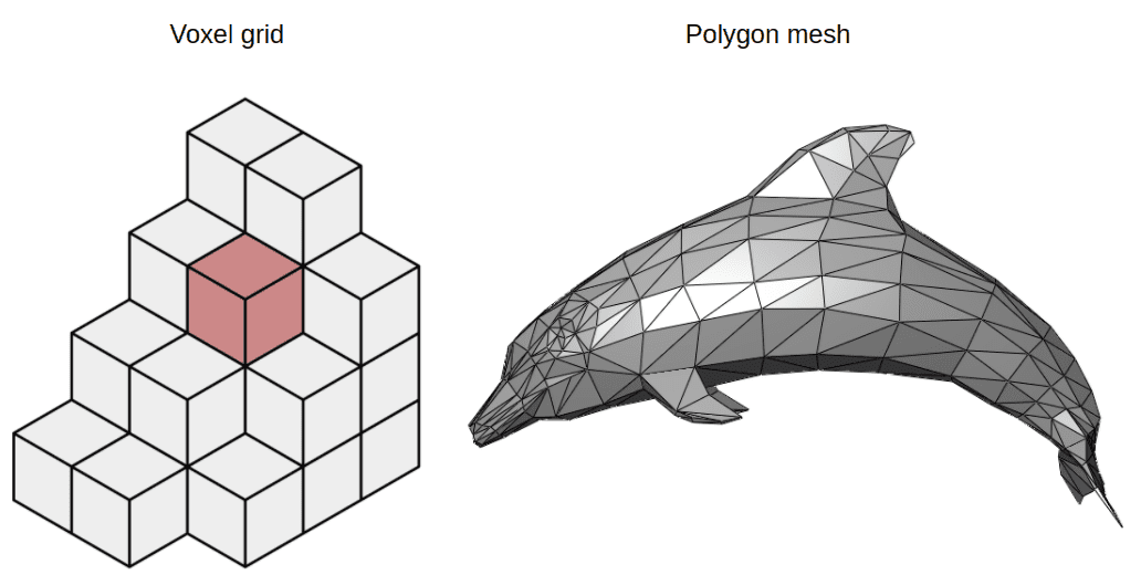 Voxels vs Polygon meshes. Source: Wikipedia on Voxels, Wikipedia on Polygon Meshes
Neural fields have gained increasing popularity in computer graphics applications as they are very efficient and compact 3D representations of objects or scenes. Why? In contrast with voxels or meshes, they are differentiable and continuous. One other advantage is that they can also have arbitrary dimensions and resolutions. Plus they are domain agnostic and do not depend on the input for each task.
At that point, you may ask: where does the name neural fields come from?
What do fields stand for?
In physics, a field is a quantity defined for all spatial and/or temporal coordinates. It can be represented as a mapping from a coordinate to a quantity , typically a scalar, a vector, or a tensor. Examples include gravitational fields and electromagnetic fields.
Next question you may ask: what are the steps to “learn” a neural field?
Steps to train a neural field
Following Xie et al. 1, the typical progress of computing neural fields can be formulated as follows:
Sample coordinates of a scene.
Feed them to a neural network to produce field quantities.
Sample the field quantities from the desired reconstruction domain of the problem.
Map the reconstruction back to the sensor domain (e.g 2D RGB images).
Calculate the reconstruction error and optimize the neural network.
 A typical neural field algorithm. Source: Xie et al. 1
For clarity, let’s use some mathematical terms to denote the process. The reconstruction is a neural field, denoted as , that maps the world coordinates to field quantities . A sensor observation is also a neural field that transforms the sensor coordinates into measurements . The forward map is a mapping between the two neural fields and is differentiable.
As a result, we can solve the following optimization problem to calculate the neural field .
The table below (Xie et al.) illustrates different applications of neural fields alongside the reconstruction and sensor domains.
 Examples of forward maps. Source: Xie et al. 1
Let’s analyze the most popular architecture of neural fields called NeRFs that solves the problem of view synthesis.
Neural Radiance Fields (NeRFs) for view synthesis
The most prominent neural field architecture is called Neural Radiance Fields or NeRFs. They were originally proposed in order to solve view synthesis. View synthesis is the task where you generate a 3D object or scene given a set of pictures from different angles (or views). View synthesis is almost equivalent to 3D reconstruction.
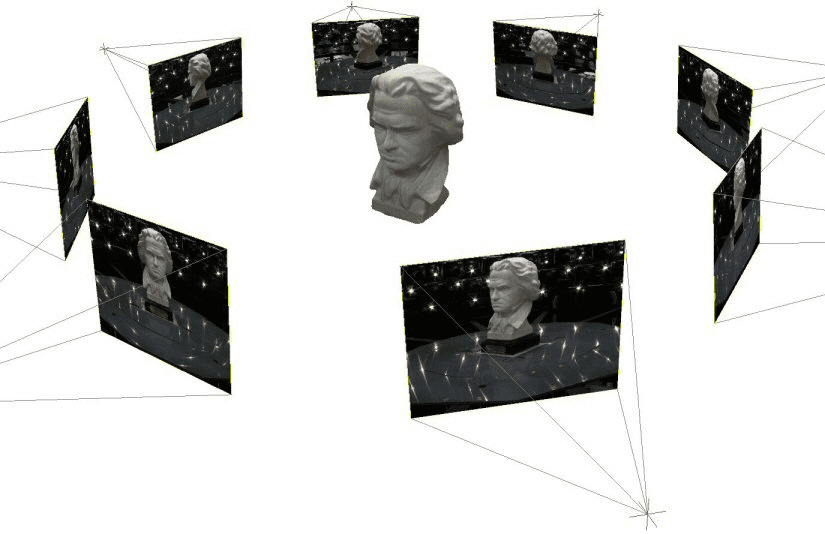 Multi-view 3D reconstruction. Source: Convex Variational Methods for Single-View and Space-Time Multi-View Reconstruction
Note that in order to fully understand NeRFs, one has to familiarize themselves with many computer graphics concepts such as volumetric rendering and ray casting. In this section, I will try to explain them as efficiently as possible but also leave a few extra resources to extend your research. If you seek for a structured course to get started with computer graphics, Computer Graphics by UC San Diego is the best one afaik
NeRFs and Neural fields terminology side by side
As I already mentioned, NeRFs are a special case of neural fields. For that reason, let’s see a side-by-side comparison. Feel free to revisit this table once we explain NeRFs in order to draw the connection between them and neural fields.
| Neural Fields | Neural Radiance Fields (NeRF) |
|---|---|
| World coordinate | Spatial location and viewing direction |
| Field quantities | Color and volume density |
| Field | MLP |
| Sensor coordinates | 2D images |
| Measurements | Radiance |
| Sensor | Digital camera |
| Forward mapping | Volume rendering |
The reason I decided to first present neural fields and then NeRFs is to understand that neural fields are a far more general framework
NeRFs explained
NeRFs as proposed by Mildenhall et al 2. accept a single continuous 5D coordinate as input, which consists of a spatial location and viewing direction . This particular point of the object/scene is fed into an MLP, which outputs the corresponding color intensities and its volume density .
The (probability) volume density indicates how much radiance (or luminance) is accumulated by a ray passing through and is a measure of the “effect” this point has on the overall scene. Intuitively, the probability volume density provides the likelihood that the predicted color value should be taken into account.
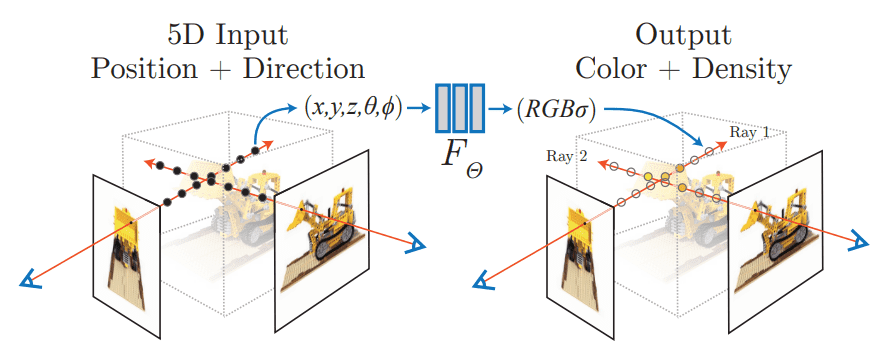 Neural Radiance Fields. Source: Mildenhall et al. 2
The power of the neural field is that it can output different representations for the same point when viewed from different angles. As a result, it can capture various lighting effects such as reflections, and transparencies, making it ideal to render different views of the same scene. This makes it a much better representation compared to voxels grid or meshes.
Training NeRFs
The problem with training these architectures is that the target density and color are not known. Therefore we need a (differentiable) method to map them back to 2D images. These images are then compared with the ground truth images formulating a rendering loss against which we can optimize the network.
 NeRFs training process. Source: Mildenhall et al. 2
As shown in the image above, volume rendering is used to map the neural field output back to 2D the image. The standard L2 loss can be computed using the input image/pixel in an autoencoder fashion. Note that volume rendering is a very common process in computer graphics. Let’s see in short how it works.
Volume rendering
When sampling coordinates from the original images, we emit rays at each pixel and sample at different timesteps, a process known as ray marching. Each sample point has a spatial location, a color, and a volume density. These are the inputs of the neural field.
A ray is a function of its origin , its direction , and its samples at timesteps . It can be formulated as . Both the volume density and the color are dependent on the ray and can be denoted as and respectively.
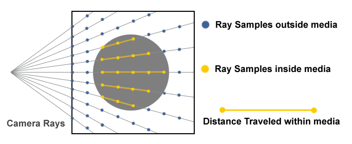 Ray Marching. Source: Creating a Volumetric Ray Marcher by Ryan Brucks
To map them back to the image, all we have to do is integrate these rays and acquire the color of each pixel.
given that and are the bound of the ray and its transmittance. The transmittance is a measure of how much the ray can penetrate the 3D space to a certain point and is defined as
The aforementioned technique, wherein you generate images or video by tracing a ray and integrating along it is also referred as neural rendering or differentiable rendering in bibliography.
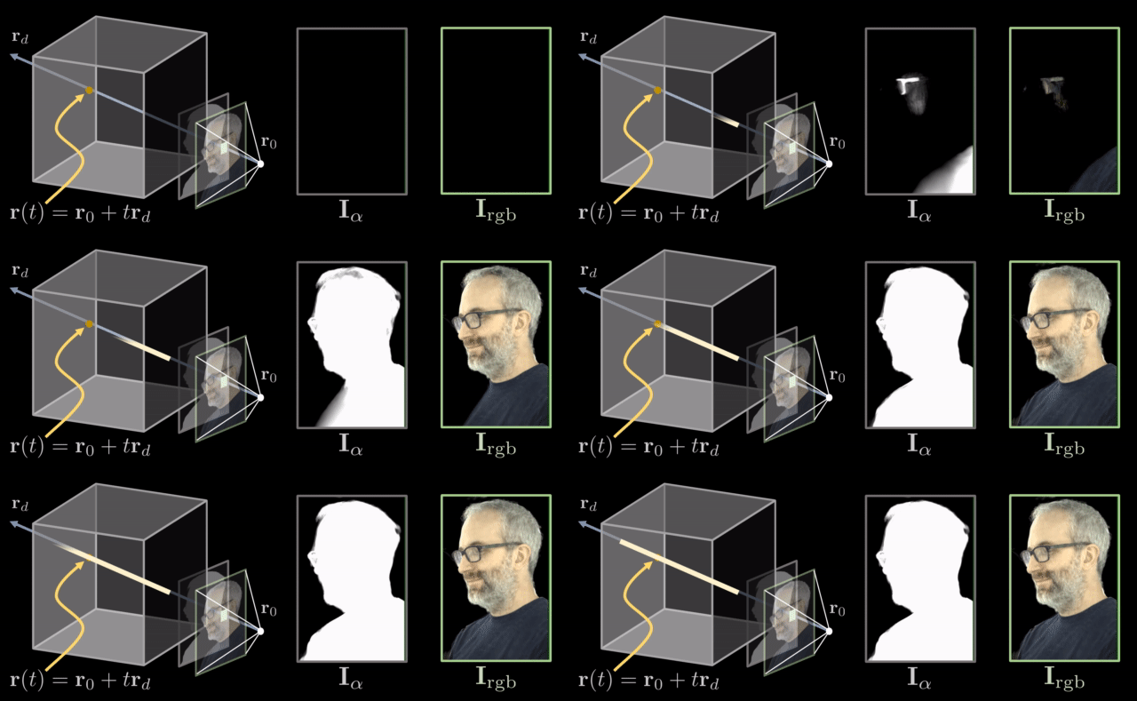 Rifferentiable ray marching. Source: Neural Volumes by Stephen Lombardi
For more details on volume rendering, check out this great lecture from Cem Yuksel and University of Utah.
For a more complete explanation of NeRFs, here is a great video by Yannic Klitcher:
A few more notes on NeRFs
The number of variations and enhancements over NeRFs is growing rapidly over the past few years. These typically fall into 4 different categories:
Aid reconstruction by computing good priors over the 3D scenes and conditioning the neural fields.
Increase the performance and complexity of training/inference. This is frequently done using hybrid representations which combine neural fields with discrete data structures.
Select better network architectures to eliminate spectral bias and efficiently compute derivatives and integrals
Manipulate neural fields representations
Note that it is almost impossible to curate a good survey of all NeRF papers. Dellaert et al 3 and Xie et al 1 are the only good sources I could find. The authors from the latter have created an excellent database of related papers as well as a very useful X account.
Instant Neural Graphics Primitives with a Multiresolution Hash Encoding
One of the most important papers following NeRFs is Instant Neural Graphics Primitives as proposed by Muller et al 4. Notably, the authors by Nvidia manage to speed up the training from hours to a couple of seconds, using a novel input representation.
The authors utilize typical neural fields, also referred to as neural graphic primitives, combined with a novel representation of the input called multiresolution hash encoding. This type of encoding permits the use of small neural networks reducing the total floating points operation needed.
As far as I know, neural graphics primitives is just a different terminology for neural fields.
Moreover, the authors suggest the use of specific GPU implementations for each task, reducing, even more, the overall computational complexity. One such proposal is to implement the entire MLP as a single CUDA kernel so that every calculation is performed in the GPU’s local cache.
Multiresolution Hash Encoding
Let’s now talk about multiresolution hash encoding, which is arguably the most important contribution of the paper. We will consider a 2D example for simplicity purposes but the following steps generalize in 3 dimensions.
Instead of training only the network parameters, we also train encoding parameters (feature vectors). These vectors are arranged into different resolution levels and stored at the vertices of a grid. Each grid corresponds to a different resolution.
Starting with a specific location on a 2D image,
We find the surrounding grids (red and blue squares in the following figure) and assign indices to the vertices of the grids by hashing their coordinates.
Because each resolution grid has a corresponding predefined hash table, we can simply look up the corresponding trainable feature vectors. Note that hashing the vertices will give the indices in the corresponding look-up tables.
To combine the feature vectors of different resolutions, we linearly interpolate them.
Next up, we concatenate them alongside other auxiliary inputs to produce the final vector.
The resulting feature vector is passed into the neural network
The whole procedure is fully differentiable. To train the encodings, the loss gradients are propagated through the MLP, concatenation, and linear interpolation, and then accumulated in the looked-up feature vectors. Also, it’s important to note that this procedure is entirely task-agnostic and can be used for different architectures and tasks besides NeRFs.
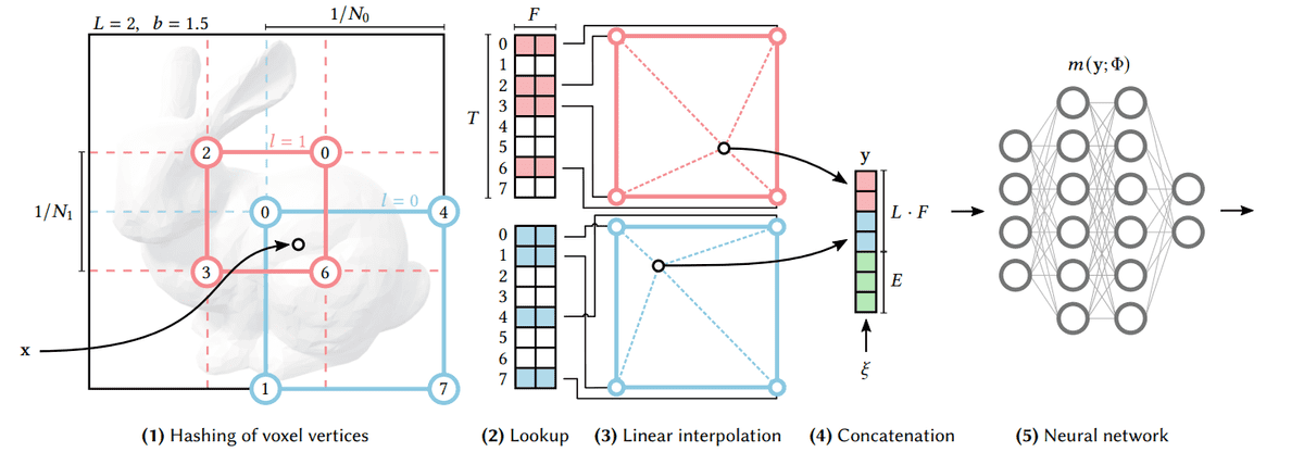 Multiresolution Hash Encoding. Source: Müller et al. 4
But what do we gain from this somewhat complicated encoding?
By training the encoding parameters alongside the network, we get a big boost in the quality of the final result.
By using multiple resolutions, we gain an automatic level of detail, meaning that the network learns both coarse and fine features.
By using hashing to associate the 3d space with feature vectors, the encoding process becomes entirely task-agnostic.
The following video provides an excellent deep dive into the paper for those interested.
Conclusion
In my opinion , NeRFs is one of the most exciting applications of neural networks of the last few years. Being able to render 3D models in a matter of seconds was simply inconceivable a couple of years ago. It won’t be long before we see these architectures enter the gaming and simulation industries.
To experiment with NeRFs, I recommend visiting the instant-ngp repo by Nvidia, install the necessary dependencies and play around by creating your own models.
If you’d like to see more articles of computer graphics, please let us know on our discord server. Finally, if you like our blogposts, feel free to support us by buying our courses or books.
References
- Xie, Yiheng, et al. Neural Fields in Visual Computing and Beyond. arXiv, 5 Apr. 2022. ↩
- Mildenhall, Ben, et al. NeRF: Representing Scenes as Neural Radiance Fields for View Synthesis. arXiv, 3 Aug. 2020↩
- Dellaert, Frank, and Lin Yen-Chen. Neural Volume Rendering: NeRF And Beyond. arXiv, 14 Jan. 2021↩
- Müller, Thomas, et al. Instant Neural Graphics Primitives with a Multiresolution Hash Encoding. ACM Transactions on Graphics, vol. 41, no. 4, July 2022, pp. 1–15↩
* Disclosure: Please note that some of the links above might be affiliate links, and at no additional cost to you, we will earn a commission if you decide to make a purchase after clicking through.