Self-supervised learning tutorial: Implementing SimCLR with pytorch lightning

In this hands-on tutorial, we will provide you with a reimplementation of SimCLR self-supervised learning method for pretraining robust feature extractors. This method is fairly general and can be applied to any vision dataset, as well as different downstream tasks.

In a previous tutorial, I wrote a bit of a background on the self-supervised learning arena. Time to get into your first project by running SimCLR on a small dataset with 100K unlabelled images called STL10.

Code is available on Github.

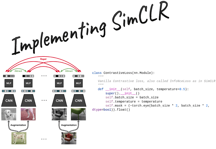
The SimCLR method: contrastive learning

Let $sim(u,v)$ note the dot product between 2 normalized $u$ and $v$ vectors (i.e. cosine similarity).

Then the loss function for a positive pair of examples (i,j) is defined as:

\ell_{i, j}=-\log \frac{\exp \left(\operatorname{sim}\left(\boldsymbol{z}_{i}, \boldsymbol{z}_{j}\right) / \tau\right)}{\sum_{k=1}^{2 N} \mathbb{1}_{[k \neq i]} \exp \left(\operatorname{sim}\left(\boldsymbol{z}_{i}, \boldsymbol{z}_{k}\right) / \tau\right)}

where $\mathbb{1}_{[k \neq i]} \in {0,1}$ is an indicator function evaluating to 1 iff $k != i$ . For more info on that check how we are going to index the similarity matrix to get the positives and the negatives.

$\tau$ denotes a temperature parameter. The final loss is computed by summing all positive pairs and divide by $2\times N = views \times batch\_size$

There are different ways to develop contrastive loss. Here we provide you with some important info.

L2 normalization and cosine similarity matrix calculation

First, one needs to apply an L2 normalization to the features, otherwise, this method does not work. L2 normalization means that the vectors are normalized such that they all lie on the surface of the unit (hyper)sphere, where the L2 norm is 1.

z_i = F.normalize(proj_1, p=2, dim=1)
z_j = F.normalize(proj_2, p=2, dim=1)

Concatenate the 2 output views in the batch dimension. Their shape will be $[2 \times batch\_size, dim]$ . Then, calculate the similarity/logits of all pairs. This can be implemented by a matrix multiplication as follows. The output shape is equal to $[batch\_size \times views, batch\_size \times views]$

def calc_similarity_batch(self, a, b):
       representations = torch.cat([a, b], dim=0)
       return F.cosine_similarity(representations.unsqueeze(1), representations.unsqueeze(0), dim=2)

Indexing the similarity matrix for the SimCLR loss function

Now we need to index the resulting matrix of size $[batch\_size \times views, batch\_size \times views]$ appropriately.

A visual illustration of SimCLR. Image from the author

Ok how the heck do we do that? I had the same question. Here the batch size is 2 images but we want to implement a solution for any batch size. If you look closely, you will see that the positive pairs are shifted from the main diagonal by 2, that is the batch size. One way to do that is torch.diag(). It takes the chosen diagonal from a matrix. The first parameter is the matrix and the second specifies the diagonal, where zero represents the main diagonal elements. We take the diagonals that are shifted by the batch size.

sim_ij = torch.diag(similarity_matrix, batch_size)
sim_ji = torch.diag(similarity_matrix, -batch_size)
positives = torch.cat([sim_ij, sim_ji], dim=0)

There are $batch\_size \times views$ positive pairs. Another example for [6,6] matrix (batch_size=3,views=2) is to have a mask that looks exactly like this:

[0., 0., 0., 1., 0., 0.],
[0., 0., 0., 0., 1., 0.],
[0., 0., 0., 0., 0., 1.],
[1., 0., 0., 0., 0., 0.],
[0., 1., 0., 0., 0., 0.],
[0., 0., 1., 0., 0., 0.]

For the denominator we need both the positive and negative pairs. So the binary mask will be the exact element wise inverse of the identity matrix.

self.mask = (~torch.eye(batch_size * 2, batch_size * 2, dtype=bool)).float()
pos_and_negatives = self.mask * similarity_matrix

Again, they are both the positives and the negatives in the denominator.

You can make out the rest of it (temperature scaling and summing the negatives from the denominator etc.):

SimCLR loss implementation

import torch
import torch.nn as nn
import torch.nn.functional as F

def device_as(t1, t2):
   """
   Moves t1 to the device of t2
   """
   return t1.to(t2.device)

class ContrastiveLoss(nn.Module):
   """
   Vanilla Contrastive loss, also called InfoNceLoss as in SimCLR paper
   """
   def __init__(self, batch_size, temperature=0.5):
       super().__init__()
       self.batch_size = batch_size
       self.temperature = temperature
       self.mask = (~torch.eye(batch_size * 2, batch_size * 2, dtype=bool)).float()

   def calc_similarity_batch(self, a, b):
       representations = torch.cat([a, b], dim=0)
       return F.cosine_similarity(representations.unsqueeze(1), representations.unsqueeze(0), dim=2)

   def forward(self, proj_1, proj_2):
       """
       proj_1 and proj_2 are batched embeddings [batch, embedding_dim]
       where corresponding indices are pairs
       z_i, z_j in the SimCLR paper
       """
       batch_size = proj_1.shape[0]
       z_i = F.normalize(proj_1, p=2, dim=1)
       z_j = F.normalize(proj_2, p=2, dim=1)

       similarity_matrix = self.calc_similarity_batch(z_i, z_j)

       sim_ij = torch.diag(similarity_matrix, batch_size)
       sim_ji = torch.diag(similarity_matrix, -batch_size)

       positives = torch.cat([sim_ij, sim_ji], dim=0)

       nominator = torch.exp(positives / self.temperature)

       denominator = device_as(self.mask, similarity_matrix) * torch.exp(similarity_matrix / self.temperature)

       all_losses = -torch.log(nominator / torch.sum(denominator, dim=1))
       loss = torch.sum(all_losses) / (2 * self.batch_size)
       return loss

Augmentations

The key to self-supervised representation learning is data augmentations. A commonly used transformation pipeline is the following:

Crop on a random scale from 7% to 100% of the image
Resize all images to 224 or other spatial dimensions.
Apply horizontal flipping with 50% probability
Apply heavy color jittering with 80% probability
Apply gaussian blur with 50% probability. Kernel size is usually around 10% of the image or less.
Convert RGB images to grayscale with 20% probability.
Normalize based on the means and variances of imagenet

This pipeline will be applied independently to each image twice and it will produce two different views that will be fed into the backbone model. In this notebook, we will use a standard resnet18.

import torch
import torchvision.transforms as T

class Augment:
   """
   A stochastic data augmentation module
   Transforms any given data example randomly
   resulting in two correlated views of the same example,
   denoted x ̃i and x ̃j, which we consider as a positive pair.
   """

   def __init__(self, img_size, s=1):
       color_jitter = T.ColorJitter(
           0.8 * s, 0.8 * s, 0.8 * s, 0.2 * s
       )
       # 10% of the image
       blur = T.GaussianBlur((3, 3), (0.1, 2.0))

       self.train_transform = torch.nn.Sequential(
           T.RandomResizedCrop(size=img_size),
           T.RandomHorizontalFlip(p=0.5),  # with 0.5 probability
           T.RandomApply([color_jitter], p=0.8),
           T.RandomApply([blur], p=0.5),
           T.RandomGrayscale(p=0.2),
           # imagenet stats
           T.Normalize(mean=[0.485, 0.456, 0.406], std=[0.229, 0.224, 0.225])
       )

   def __call__(self, x):
       return self.train_transform(x), self.train_transform(x)

Below are 4 different views of the same image by applying the same stochastic pipeline:

4 different augmentation of the same with the same pipeline. Image by author

To visualize them you need to undo the mean-std normalization and put the color channels in the last dimension:

def imshow(img):
   """
   shows an imagenet-normalized image on the screen
   """
   mean = torch.tensor([0.485, 0.456, 0.406], dtype=torch.float32)
   std = torch.tensor([0.229, 0.224, 0.225], dtype=torch.float32)
   unnormalize = T.Normalize((-mean / std).tolist(), (1.0 / std).tolist())
   npimg = unnormalize(img).numpy()
   plt.imshow(np.transpose(npimg, (1, 2, 0)))
   plt.show()

dataset = STL10("./", split='train', transform=Augment(96), download=True)
# 99 is the image id 
imshow(dataset[99][0][0])
imshow(dataset[99][0][0])
imshow(dataset[99][0][0])
imshow(dataset[99][0][0])

Modify Resnet18 and define parameter groups

One important step to run the simclr is to remove the last fully connected layer. We will replace it with an identity function. Then, we need to add the projection head (another MLP) that will be used only for the self-supervised pretraining stage. To do so, we need to be aware of the dimension of the features of our model. In particular, resnet18 outputs a 512-dim vector while resnet50 outputs a 2048-dim vector. The projection MLP would transform it to the embedding vector size which is 128, based on the official paper.

To optimize SSL models we use heavy regularization techniques, like weight decay. To avoid performance deterioration we need to exclude the weight decay from the batch normalization layers.

import pytorch_lightning as pl
import torch
import torch.nn.functional as F
from pl_bolts.optimizers.lr_scheduler import LinearWarmupCosineAnnealingLR
from torch.optim import SGD, Adam

class AddProjection(nn.Module):
   def __init__(self, config, model=None, mlp_dim=512):
       super(AddProjection, self).__init__()
       embedding_size = config.embedding_size
       self.backbone = default(model, models.resnet18(pretrained=False, num_classes=config.embedding_size))
       mlp_dim = default(mlp_dim, self.backbone.fc.in_features)
       print('Dim MLP input:',mlp_dim)
       self.backbone.fc = nn.Identity()

       # add mlp projection head
       self.projection = nn.Sequential(
           nn.Linear(in_features=mlp_dim, out_features=mlp_dim),
           nn.BatchNorm1d(mlp_dim),
           nn.ReLU(),
           nn.Linear(in_features=mlp_dim, out_features=embedding_size),
           nn.BatchNorm1d(embedding_size),
       )

   def forward(self, x, return_embedding=False):
       embedding = self.backbone(x)
       if return_embedding:
           return embedding
       return self.projection(embedding)

The next step is to separate the models’ parameters into 2 groups.

The purpose of the second group is to remove weight decay from batch normalization layers. In the case of using the LARS optimizer, you also need to remove weight decay from biases. One way to achieve that is the following function:

def define_param_groups(model, weight_decay, optimizer_name):
   def exclude_from_wd_and_adaptation(name):
       if 'bn' in name:
           return True
       if optimizer_name == 'lars' and 'bias' in name:
           return True

   param_groups = [
       {
           'params': [p for name, p in model.named_parameters() if not exclude_from_wd_and_adaptation(name)],
           'weight_decay': weight_decay,
           'layer_adaptation': True,
       },
       {
           'params': [p for name, p in model.named_parameters() if exclude_from_wd_and_adaptation(name)],
           'weight_decay': 0.,
           'layer_adaptation': False,
       },
   ]
   return param_groups

I am not using the LARS optimizer in this tutorial but if you plan to use it here is an implementation that I use as a reference.

SimCLR training logic

Here we will implement the whole training logic of SimCLR. Take 2 views, forward them to get the embedding projections, and calculate the SimCLR loss.

We can wrap up the SimCLR training with one class using Pytorch lightning that encapsulates all the training logic. In its simplest form, we need to implement the training_step method that gets as input a batch from the dataloader. You can think of it as calling batch = next(iter(dataloader)) in each step. Next comes the configure_optimizers method which binds the model with the optimizer and the training scheduler. I used an already implemented scheduler from PyTorch lightning bolts (another small package in the lightning ecosystem). Essentially, we gradually increase the learning rate to its base value and then we do cosine annealing.

class SimCLR_pl(pl.LightningModule):
   def __init__(self, config, model=None, feat_dim=512):
       super().__init__()
       self.config = config
       self.augment = Augment(config.img_size)
       self.model = AddProjection(config, model=model, mlp_dim=feat_dim)

       self.loss = ContrastiveLoss(config.batch_size, temperature=self.config.temperature)

   def forward(self, X):
       return self.model(X)

   def training_step(self, batch, batch_idx):
       x, labels = batch
       x1, x2 = self.augment(x)
       z1 = self.model(x1)
       z2 = self.model(x2)
       loss = self.loss(z1, z2)
       self.log('Contrastive loss', loss, on_step=True, on_epoch=True, prog_bar=True, logger=True)
       return loss

   def configure_optimizers(self):
       max_epochs = int(self.config.epochs)
       param_groups = define_param_groups(self.model, self.config.weight_decay, 'adam')
       lr = self.config.lr
       optimizer = Adam(param_groups, lr=lr, weight_decay=self.config.weight_decay)

       print(f'Optimizer Adam, '
             f'Learning Rate {lr}, '
             f'Effective batch size {self.config.batch_size * self.config.gradient_accumulation_steps}')

       scheduler_warmup = LinearWarmupCosineAnnealingLR(optimizer, warmup_epochs=10, max_epochs=max_epochs,
                                                        warmup_start_lr=0.0)

       return [optimizer], [scheduler_warmup]

Gradient accumulation and effective batch size

Here it is crucial to highlight the importance of using a big batch size. This method is heavily dependent on a large batch size to push away from the 2 views of the same image (positives). To do that on a restricted budget we can use gradient accumulation. We average the gradients of $N$ steps and then update the model, instead of updating after each forward-backward pass.

Thus, now it should make complete sense that the effective batch is: $batch\_size\_per\_gpu * accumulation\_steps * number\_of\_gpus$ . This is super easy to do in PyTorch lightning using a callback function.

“In computer programming, a callback is a reference to executable code or a piece of executable code that is passed as an argument to other code. This allows a lower-level software layer to call a subroutine (or function) defined in a higher-level layer.” ~ StackOverflow

from pytorch_lightning.callbacks import GradientAccumulationScheduler
accumulator = GradientAccumulationScheduler(scheduling={0: train_config.gradient_accumulation_steps})

# then pass it in the Trainer class init

Main SimCLR pretraining script

The main script just collects everything together and initializes the Trainer class of PyTorch lightning. You can then run it on a single or multiple GPUs. Note that in the snippet below,I am reading all the available GPUs of the system.

import torch
from pytorch_lightning import Trainer
import os
from pytorch_lightning.callbacks import GradientAccumulationScheduler
from pytorch_lightning.callbacks import ModelCheckpoint
from torchvision.models import  resnet18

available_gpus = len([torch.cuda.device(i) for i in range(torch.cuda.device_count())])
save_model_path = os.path.join(os.getcwd(), "saved_models/")
print('available_gpus:',available_gpus)
filename='SimCLR_ResNet18_adam_'
resume_from_checkpoint = False
train_config = Hparams()

reproducibility(train_config)
save_name = filename + '.ckpt'

model = SimCLR_pl(train_config, model=resnet18(pretrained=False), feat_dim=512)

data_loader = get_stl_dataloader(train_config.batch_size)

accumulator = GradientAccumulationScheduler(scheduling={0: train_config.gradient_accumulation_steps})
checkpoint_callback = ModelCheckpoint(filename=filename, dirpath=save_model_path,every_n_val_epochs=2,
                                       save_last=True, save_top_k=2,monitor='Contrastive loss_epoch',mode='min')

if resume_from_checkpoint:
    trainer = Trainer(callbacks=[accumulator, checkpoint_callback],
        gpus=available_gpus,
        max_epochs=train_config.epochs,
        resume_from_checkpoint=train_config.checkpoint_path)
else:
    trainer = Trainer(callbacks=[accumulator, checkpoint_callback],
        gpus=available_gpus,
        max_epochs=train_config.epochs)

trainer.fit(model, data_loader)
trainer.save_checkpoint(save_name)
# google colab only
from google.colab import files
files.download(save_name)

Finetuning

Ok, we trained a model. Now it’s time for fine-tuning. We will use the PyTorch lightning module class to encapsulate the logic. I am taking the pretrained resnet18 backbone, without the projection head, and I am only adding one linear layer on top. I am fine tuning the whole network. No augmentations are applied here. They would only delay the training. Instead, we would like to quantify the performance against pretrained weights on imagenet and random initialization.

import pytorch_lightning as pl
import torch
from torch.optim import SGD

class SimCLR_eval(pl.LightningModule):
   def __init__(self, lr, model=None, linear_eval=False):
       super().__init__()
       self.lr = lr
       self.linear_eval = linear_eval
       if self.linear_eval:
            model.eval()
       self.mlp = torch.nn.Sequential(
            torch.nn.Linear(512,10), # only one linear layer on top
       )

       self.model = torch.nn.Sequential(
            model, self.mlp
       )
       self.loss = torch.nn.CrossEntropyLoss()

   def forward(self, X):
       return self.model(X)

   def training_step(self, batch, batch_idx):
       x, y = batch
       z = self.forward(x)
       loss = self.loss(z, y)
       self.log('Cross Entropy loss', loss, on_step=True, on_epoch=True, prog_bar=True, logger=True)

       predicted = z.argmax(1)
       acc = (predicted == y).sum().item() / y.size(0)
       self.log('Train Acc', acc, on_step=False, on_epoch=True, prog_bar=True, logger=True)

       return loss


   def validation_step(self, batch, batch_idx):
       x, y = batch
       z = self.forward(x)
       loss = self.loss(z, y)
       self.log('Val CE loss', loss, on_step=True, on_epoch=True, prog_bar=False, logger=True)

       predicted = z.argmax(1)
       acc = (predicted == y).sum().item() / y.size(0)
       self.log('Val Accuracy', acc, on_step=True, on_epoch=True, prog_bar=True, logger=True)

       return loss

   def configure_optimizers(self):
       if self.linear_eval:
           print(f"\n\n Attention! Linear evaluation \n")
           optimizer = SGD(self.mlp.parameters(), lr=self.lr, momentum=0.9)
       else:
           optimizer = SGD(self.model.parameters(), lr=self.lr, momentum=0.9)
       return [optimizer]

Importantly, STL10 is a subset of imagenet so transfer learning from imagenet is expected to work very well.

Method	Finetunning the whole network, Validation Accuracy	Linear evaluation. Validation Accuracy
SimCLR pretraining on STL10 unlabelled split	75.1%	73.2 %
Imagenet pretraining (1M)	87.9%	78.6 %
Random initialization	50.6 %	-

In all cases the model overfits during finetuning. Remember no augmentations were applied.

Conclusion

Even with an unfair evaluation compared to pretrained weights from imagenet, contrastive self-supervised learning demonstrates some super promising results. There are many other self-supervised methods to play with, but SimCLR is the baseline.

To wrap up, we explored how to build step by step the SimCLR loss function and launch a training script without too much boilerplate code with Pytorch-lightning. Even though there is a gap between SimCLR learned representations, latest state-of-the-art methods are catching up and even surpass imagenet-learned features in many domains.

Thanks for your interest in AI and stay positive!

* Disclosure: Please note that some of the links above might be affiliate links, and at no additional cost to you, we will earn a commission if you decide to make a purchase after clicking through.