BYOL tutorial: self-supervised learning on CIFAR images with code in Pytorch

After presenting SimCLR, a contrastive self-supervised learning framework, I decided to demonstrate another infamous method, called BYOL. Bootstrap Your Own Latent (BYOL), is a new algorithm for self-supervised learning of image representations. BYOL has two main advantages:

It does not explicitly use negative samples. Instead, it directly minimizes the similarity of representations of the same image under a different augmented view (positive pair). Negative samples are images from the batch other than the positive pair.
As a result, BYOL is claimed to require smaller batch sizes, which makes it an attractive choice.

Below, you can examine the method. Unlike the original paper, I call the online network student and the target network teacher.

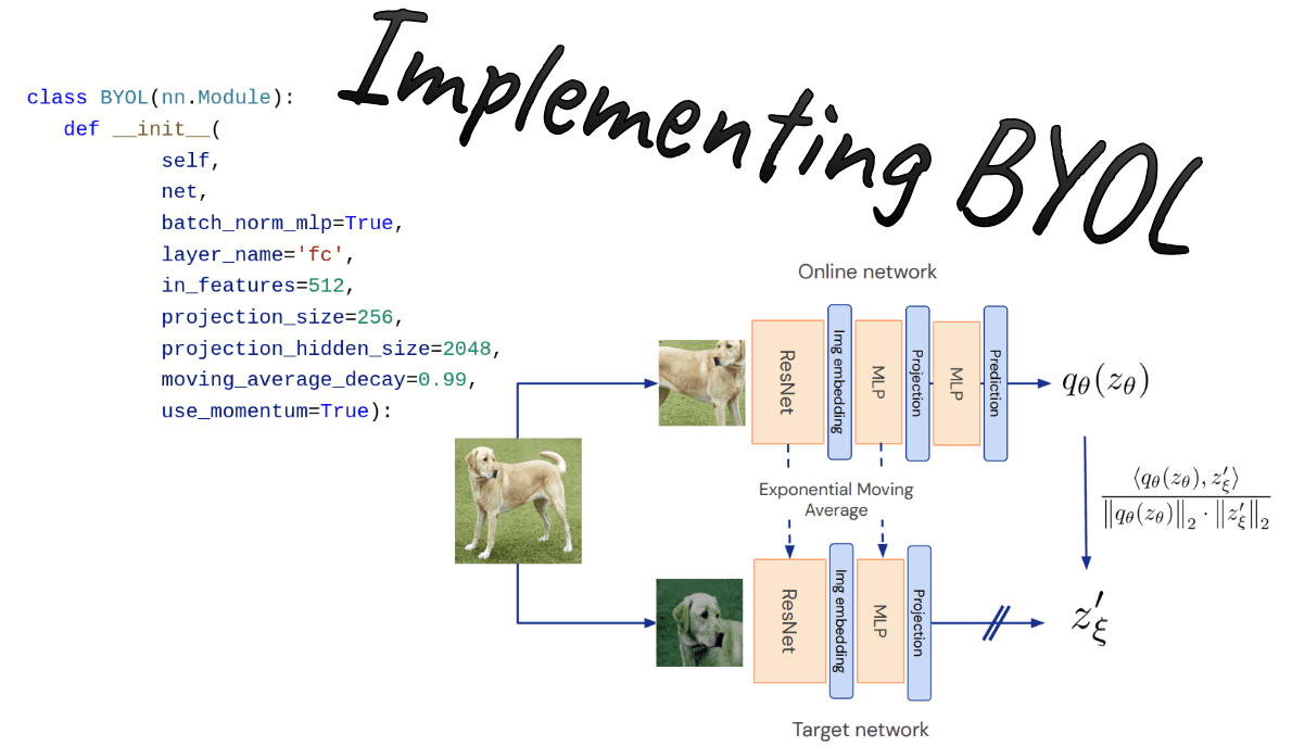
Overview of BYOL method. Source: BYOL paper

Online network aka student: compared to SimCLR, there is a second MLP, called predictor, which makes the whole method asymmetric. Asymmetric compared to what? Well, to the teacher model (target network).

Why is that important?

Because the teacher model is updated only through exponential moving average (EMA) from the student’s parameters. Ultimately, at each iteration, a tiny percentage (less than 1%) of the parameters of the student is passed to the teacher. Thus, gradients flow only through the student network. This can be implemented as:

class EMA():
   def __init__(self, alpha):
       super().__init__()
       self.alpha = alpha

   def update_average(self, old, new):
       if old is None:
           return new
       return old * self.alpha + (1 - self.alpha) * new

ema = EMA(0.99)
for student_params, teacher_params in zip(student_model.parameters(),teacher_model.parameters()):
         old_weight, up_weight = teacher_params.data, student_params.data
         teacher_params.data = ema.update_average(old_weight, up_weight)

Another key difference between Simclr and BYOL is the loss function.

Loss function

The predictor MLP is only applied to the student, making the architecture asymmetric. This is a key design choice to avoid mode collapse. Mode collapse here would be to output the same projection for all the inputs.

Overview of BYOL method. Source: BYOL paper

Finally, the authors defined the following mean squared error between the L2-normalized predictions and target projections:

\mathcal{L}_{\theta, \xi} \triangleq\left\|\bar{q}_{\theta}\left(z_{\theta}\right)-\bar{z}_{\xi}^{\prime}\right\|_{2}^{2}=2-2 \cdot \frac{\left\langle q_{\theta}\left(z_{\theta}\right), z_{\xi}^{\prime}\right\rangle}{\left\|q_{\theta}\left(z_{\theta}\right)\right\|_{2} \cdot\left\|z_{\xi}^{\prime}\right\|_{2}} .

The L2 loss can be implemented as follows. L2 normalization is applied beforehand.

import torch
import torch.nn.functional as F

def loss_fn(x, y):
   # L2 normalization
   x = F.normalize(x, dim=-1, p=2)
   y = F.normalize(y, dim=-1, p=2)
   return 2 - 2 * (x * y).sum(dim=-1)

Code is available on GitHub

Tracking down what’s happening in self-supervised pretraining: KNN accuracy

Nonetheless, the loss in self-supervised learning is not a reliable metric to track. What I found out to be the best way to track what’s happening while training, is to measure the ΚΝΝ accuracy.

The critical advantage of using KNN is that we don't have to train a linear classifier on top each time, so it’s faster and completely unsupervised.

Note: Measuring KNN only applies to image classification, but you get the idea. For this purpose, I made a class to encapsulate the logic of KNN in our context:

import numpy as np
import torch
from sklearn.model_selection import cross_val_score
from sklearn.neighbors import KNeighborsClassifier
from torch import nn

class KNN():
   def __init__(self, model, k, device):
       super(KNN, self).__init__()
       self.k = k
       self.device = device
       self.model = model.to(device)
       self.model.eval()

   def extract_features(self, loader):
       """
       Infer/Extract features from a trained model
       Args:
           loader: train or test loader
       Returns: 3 tensors of all:  input_images, features, labels
       """
       x_lst = []
       features = []
       label_lst = []

       with torch.no_grad():
           for input_tensor, label in loader:
               h = self.model(input_tensor.to(self.device))
               features.append(h)
               x_lst.append(input_tensor)
               label_lst.append(label)

           x_total = torch.stack(x_lst)
           h_total = torch.stack(features)
           label_total = torch.stack(label_lst)

           return x_total, h_total, label_total

   def knn(self, features, labels, k=1):
       """
       Evaluating knn accuracy in feature space.
       Calculates only top-1 accuracy (returns 0 for top-5)
       Args:
           features: [... , dataset_size, feat_dim]
           labels: [... , dataset_size]
           k: nearest neighbours
       Returns: train accuracy, or train and test acc
       """
       feature_dim = features.shape[-1]
       with torch.no_grad():
           features_np = features.cpu().view(-1, feature_dim).numpy()
           labels_np = labels.cpu().view(-1).numpy()
           # fit
           self.cls = KNeighborsClassifier(k, metric="cosine").fit(features_np, labels_np)
           acc = self.eval(features, labels)


       return acc


   def eval(self, features, labels):
     feature_dim = features.shape[-1]
     features = features.cpu().view(-1, feature_dim).numpy()
     labels = labels.cpu().view(-1).numpy()
     acc = 100 * np.mean(cross_val_score(self.cls, features, labels))
     return acc

   def _find_best_indices(self, h_query, h_ref):
       h_query = h_query / h_query.norm(dim=1).view(-1, 1)
       h_ref = h_ref / h_ref.norm(dim=1).view(-1, 1)
       scores = torch.matmul(h_query, h_ref.t())  # [query_bs, ref_bs]
       score, indices = scores.topk(1, dim=1)  # select top k best
       return score, indices

   def fit(self, train_loader, test_loader=None):
       with torch.no_grad():
           x_train, h_train, l_train = self.extract_features(train_loader)
           train_acc = self.knn(h_train, l_train, k=self.k)

           if test_loader is not None:
               x_test, h_test, l_test = self.extract_features(test_loader)
               test_acc = self.eval(h_test, l_test)
               return train_acc, test_acc

Now we can focus on the method and BYOL model.

Modify resnet: add MLP projection heads

We will start with a base model (resnet18) and modify it for self-supervised learning. The last layer that normally does the classification is replaced with an identity function. The output features of resnet18 will be fed to the MLP projector.

import copy
import torch
from torch import nn
import torch.nn.functional as F

class MLP(nn.Module):
   def __init__(self, dim, embedding_size=256, hidden_size=2048, batch_norm_mlp=False):
       super().__init__()
       norm = nn.BatchNorm1d(hidden_size) if batch_norm_mlp else nn.Identity()
       self.net = nn.Sequential(
           nn.Linear(dim, hidden_size),
           norm,
           nn.ReLU(inplace=True),
           nn.Linear(hidden_size, embedding_size)
       )

   def forward(self, x):
       return self.net(x)

class AddProjHead(nn.Module):
   def __init__(self, model, in_features, layer_name, hidden_size=4096,
                embedding_size=256, batch_norm_mlp=True):
       super(AddProjHead, self).__init__()
       self.backbone = model
       # remove last layer 'fc' or 'classifier'
       setattr(self.backbone, layer_name, nn.Identity())
       self.backbone.conv1 = torch.nn.Conv2d(3, 64, kernel_size=3, stride=1, padding=1, bias=False)
       self.backbone.maxpool = torch.nn.Identity()
       # add mlp projection head
       self.projection = MLP(in_features, embedding_size, hidden_size=hidden_size, batch_norm_mlp=batch_norm_mlp)

   def forward(self, x, return_embedding=False):
       embedding = self.backbone(x)
       if return_embedding:
           return embedding
       return self.projection(embedding)

I also replaced the first conv layer of resnet18 from 7x7 to 3x3 convolution since we are playing with 32x32 images (CIFAR-10).

Code is available on GitHub. If you are planning to solidify your Pytorch knowledge, there are two amazing books that we highly recommend: Deep learning with PyTorch from Manning Publications and Machine Learning with PyTorch and Scikit-Learn by Sebastian Raschka. You can always use the 35% discount code blaisummer21 for all Manning’s products.

The actual BYOL method

So far I presented all the important components to reach this point. Now we will build the BYOL module with our beloved student and teacher networks. Notice that the student predictor MLP and projector are identical.

My implementation of BYOL was based on lucidrains’ repo. I modified it to make it more simple and play around with it.

class BYOL(nn.Module):
   def __init__(
           self,
           net,
           batch_norm_mlp=True,
           layer_name='fc',
           in_features=512,
           projection_size=256,
           projection_hidden_size=2048,
           moving_average_decay=0.99,
           use_momentum=True):
       """
       Args:
           net: model to be trained
           batch_norm_mlp: whether to use batchnorm1d in the mlp predictor and projector
           in_features: the number features that are produced by the backbone net i.e. resnet
           projection_size: the size of the output vector of the two identical MLPs
           projection_hidden_size: the size of the hidden vector of the two identical MLPs
           augment_fn2: apply different augmentation the second view
           moving_average_decay: t hyperparameter to control the influence in the target network weight update
           use_momentum: whether to update the target network
       """
       super().__init__()
       self.net = net
       self.student_model = AddProjHead(model=net, in_features=in_features,
                                        layer_name=layer_name,
                                        embedding_size=projection_size,
                                        hidden_size=projection_hidden_size,
                                        batch_norm_mlp=batch_norm_mlp)
       self.use_momentum = use_momentum
       self.teacher_model = self._get_teacher()
       self.target_ema_updater = EMA(moving_average_decay)
       self.student_predictor = MLP(projection_size, projection_size, projection_hidden_size)


   @torch.no_grad()
   def _get_teacher(self):
       return copy.deepcopy(self.student_model)


   @torch.no_grad()
   def update_moving_average(self):
       assert self.use_momentum, 'you do not need to update the moving average, since you have turned off momentum ' \
                                 'for the target encoder '
       assert self.teacher_model is not None, 'target encoder has not been created yet'

       for student_params, teacher_params in zip(self.student_model.parameters(), self.teacher_model.parameters()):
         old_weight, up_weight = teacher_params.data, student_params.data
         teacher_params.data = self.target_ema_updater.update_average(old_weight, up_weight)

   def forward(
           self,
           image_one, image_two=None,
           return_embedding=False):
       if return_embedding or (image_two is None):
           return self.student_model(image_one, return_embedding=True)

       # student projections: backbone + MLP projection
       student_proj_one = self.student_model(image_one)
       student_proj_two = self.student_model(image_two)

       # additional student's MLP head called predictor
       student_pred_one = self.student_predictor(student_proj_one)
       student_pred_two = self.student_predictor(student_proj_two)

       with torch.no_grad():
           # teacher processes the images and makes projections: backbone + MLP
           teacher_proj_one = self.teacher_model(image_one).detach_()
           teacher_proj_two = self.teacher_model(image_two).detach_()


       loss_one = loss_fn(student_pred_one, teacher_proj_one)
       loss_two = loss_fn(student_pred_two, teacher_proj_two)       

       return (loss_one + loss_two).mean()

For CIFAR-10 it’s enough to use 2048 as a hidden dimension and 256 as the embedding dimension. We will train a resnet18 that outputs 512 features for 100 epochs. The parts of the code that refer to data loading and augmentations are omitted to increase readability. You can look them up in the code.

You can use the Adam optimizer ( $lr=3 * 10^{-4}$ of course) or LARS with $lr=0.1$ . The reported results are with Adam, but I also validated that KNN increases in the first epochs with LARS.

The only thing that will be changed in the train code is the EMA update.

def training_step(model, data):
   (view1, view2), _ = data
   loss = model(view1.cuda(), view2.cuda())
   return loss

def train_one_epoch(model, train_dataloader, optimizer):
   model.train()
   total_loss = 0.
   num_batches = len(train_dataloader)
   for data in train_dataloader:
       optimizer.zero_grad()
       loss = training_step(model, data)
       loss.backward()
       optimizer.step()
       # EMA update
       model.update_moving_average()

       total_loss += loss.item()


   return total_loss/num_batches

Let’s jump at the results!

Results: KNN accuracy VS pretraining epochs

KNN accuracy every 4 epochs. Image by author

Isn’t it amazing that without any labels we can reach a validation accuracy of 70%? I found this amazing, especially for this method that seems to be less sensitive to the batch size.

But why does the batch size has an effect here? Isn’t it supposed to be not using negative paris? Where does the dependence of the batch size come from?

Short answer: Well, it’s batch normalization in the MLP layers!

Here is the experiments I made to cross-check it.

A note on batch norm in MLP networks and EMA momentum

I was curious to observe the mode collapse without batch normalization. You can try that by yourself by setting:

model = BYOL(model, in_features=512, batch_norm_mlp=False)

I observed that the L2 distance goes to almost zero from the very first epochs:

Epoch 0: loss:0.06423207696957084
Epoch 8: loss:0.005584242034894534
Epoch 20: loss:0.005460431350347323

The loss goes to roughly zero and KNN stops increasing (35% VS 60% in the normal setup). That’s why it’s claimed that BYOL implicitly uses a form of contrastive learning by leveraging the batch statistics in the MLPs. Here is the KNN accuracy:

Mode collapse in BYOL by removing batch norm in MLPs. Image by author

I am well aware of papers that show that batch statistics are not the only condition for BYOL to work. This is an experimental post, so I am not going to play that game. I was just curious to observe mode collapse here.

Conclusion

For a more detailed explanation of the method check Yannic’s video on BYOL:

In this tutorial, we implemented BYOL step by step and pretrained on CIFAR10. We observe the massive increase in KNN accuracy by matching the representations of the same image. A random classifier would have 10% and with 100 epochs we reach 70% KNN validation accuracy without any labels. How cool is that?

To learn more about self-supervised learning, stay tuned! Support us by social media sharing, making a donation, or buying our Deep learning in Production book. It would be highly appreciated.

* Disclosure: Please note that some of the links above might be affiliate links, and at no additional cost to you, we will earn a commission if you decide to make a purchase after clicking through.