How to Generate Images using Autoencoders

You know what would be cool? If we didn’t need all those labeled data to train our models. I mean labeling and categorizing data requires too much work. Unfortunately, most of the existing models from support vector machines to convolutional neural networks can’t be trained without them.

Except of a small group of algorithms that they can. Intrigued? That’s called Unsupervised Learning. Unsupervised Learning infers a function from unlabeled data by its own. The most famous unsupervised algorithms are K-Means, which has been used widely for clustering data into groups and PCA, which is the go to solution for dimensionality reduction. K-Means and PCA are probably the two best machine learning algorithms ever conceived. And what makes them even better is their simplicity. I mean if you grasp them, you will be all like: “Why didn’t I think of that sooner?”

The next question that comes into our minds is: "Is there an unsupervised neural network? ". You probably know the answer from the title of the post.

Autoencoders.

For the better comprehension of autoencoders, I will present some code alongside with the explanation. Note that we will use Pytorch to build and train our model.

import torch
from torch import nn, optim
from torch.autograd import Variable
from torch.nn import functional as F

Autoencoders are simple neural networks that their output is their input. Simple as that. Their goal is to learn how to reconstruct the input-data. But how is it helpful? The trick is their structure. The first part of the network is what we refer to as the Encoder. It receives the input and it encodes it in a latent space of a lower dimension. The second part (the Decoder) takes that vector and decode it in order to produce the original input.

Autoencoder Neural Networks for Outlier Correction in ECG- Based Biometric Identification

The latent vector in the middle is what we want, as it is a compressed representation of the input. And the applications are plentiful such as:

• Compression

• Dimensionality Reduction

Furthermore, it is clear that we can apply them to reproduce the same but a little different or even better data. Examples are:

• Data Denoising: Feed them with a noisy image and train them to output the same image but without the noise

• Training data augmentation

• Anomaly Detection: Train them on a single class so that every anomaly gives a large reconstruction error.

Autoencoders however, face the same few problems as most neural networks. They tend to overfit and they suffer from the vanishing gradient problem. Is there a solution?

Variational Autoencoder (VAE)

The variational autoencoder is a pretty good and elegant effort. It essentially adds randomness but not quite exactly.

Let’s explain it further. Variational autoencoders are trained to learn the probability distribution that models the input-data and not the function that maps the input and the output. It then samples points from this distribution and feed them to the decoder to generate new input data samples. But wait a minute. When I hear about probability distribution there is only one thing comes to mind: Bayes. And yes, Bayesian rule is the major principle once more. By the way, I do not mean to exaggerate, but Bayes formula is the single best equation ever created. And I am not kidding. It is everywhere. If you do not know what is, please look it up. Ditch that article and learn what Bayes is. I’ll forgive you.

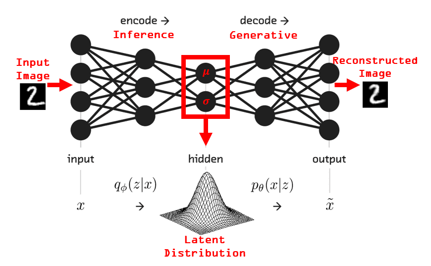
Back to variational autoencoders. I think the following image clear things up:

Texture Synthesis with Recurrent Variational Auto-Encoder

There you have it. A stochastic neural network. Before we build an example our own that generates new images, it is appropriate to discuss a few more details.

One of the key aspects of VAE is the loss function. Most commonly, it consists of two components. The reconstruction loss measures how different the reconstructed data are from the original data (binary cross entropy for example). The KL-divergence tries to regularize the process and keep the reconstructed data as diverse as possible.

def loss_function(recon_x, x, mu, logvar) -> Variable:
    BCE = F.binary_cross_entropy(recon_x, x.view(-1, 784))
    KLD = -0.5 * torch.sum(1 + logvar - mu.pow(2) - logvar.exp())
    KLD /= BATCH_SIZE * 784

    return BCE + KLD

Another important aspect is how to train the model. The difficulty occurs because the variables are note deterministic but random and gradient descent normally doesn’t work that way. To address it, we use reparameterization. The latent vector (z) will be equal with the learned mean (μ) of our distribution plus the learned standard deviation (σ) times epsilon (ε), where ε follows the normal distribution. We reparameterize the samples so that the randomness is independent of the parameters.

def reparameterize(self, mu: Variable, logvar: Variable) -> Variable:

        #mu :  mean matrix
        #logvar :  variance matrix
        if self.training:
            std = logvar.mul(0.5).exp_()  # type: Variable
            eps = Variable(std.data.new(std.size()).normal_())
            return eps.mul(std).add_(mu)
        else:
            return mu

Image Generation with AutoEncoders

In our example, we will try to generate new images using a variational auto encoder. We are going to use the MNIST dataset and the reconstructed images will be handwritten numeric digits. As I already told you, I use Pytorch as a framework, for no particular reason, other than familiarization. First, we should define our layers.

def __init__(self):
        super(VAE, self).__init__()

        # ENCODER
        self.fc1 = nn.Linear(784, 400)
        self.relu = nn.ReLU()
        self.fc21 = nn.Linear(400, 20)  # mu layer
        self.fc22 = nn.Linear(400, 20)  # logvariance layer

        # DECODER
        self.fc3 = nn.Linear(20, 400)
        self.fc4 = nn.Linear(400, 784)
        self.sigmoid = nn.Sigmoid()

As you can see , we will use a very simple network with just Dense (Linear in pytorch's case) layers. The next step is to build the function that run the encoder and decoder.

def encode(self, x: Variable) -> (Variable, Variable):
        h1 = self.relu(self.fc1(x))
        return self.fc21(h1), self.fc22(h1)

 def decode(self, z: Variable) -> Variable:
        h3 = self.relu(self.fc3(z))
        return self.sigmoid(self.fc4(h3))

def forward(self, x: Variable) -> (Variable, Variable, Variable):
    mu, logvar = self.encode(x.view(-1, 784))
    z = self.reparameterize(mu, logvar)
    return self.decode(z), mu, logvar

It's just a few lines of python code. No big deal. Finally we get to train our model and see our generated images.

Quick reminder: Pytorch has a dynamic graph in contrast to tensorflow, which means that the code is running on the fly. There is no need to create the graph and then compile an execute it, Tensorflow has recently introduce the above functionality with its eager execution mode.

optimizer = optim.Adam(model.parameters(), lr=1e-3)

def train(epoch):
    model.train()
    train_loss = 0

    for batch_idx, (data, _) in enumerate(train_loader):
        data = Variable(data)
        optimizer.zero_grad()
        recon_batch, mu, logvar = model(data)
        loss = loss_function(recon_batch, data, mu, logvar)
        loss.backward()
        train_loss += loss.data[0]
        optimizer.step()


def test(epoch):
    model.eval()
    test_loss = 0

    for i, (data, _) in enumerate(test_loader):
        data = Variable(data, volatile=True)
        recon_batch, mu, logvar = model(data)
        test_loss += loss_function(recon_batch, data, mu, logvar).data[0]

for epoch in range(1, EPOCHS + 1):
    train(epoch)
    test(epoch)

When the training is completed, we execute the test function to examine how well the model works. As a matter of fact it did a pretty good and the constructed images are amost identical with the original and i am sure no one could be able to tell them apart without knowing the whole story.

The image below shows the original photos in the first row and the produced in the second one.

Quite good, isn't it?

For more details on AutoEncoders, you should check the module 5 of the Deep Learning with Tensorflow course by edX.

Before we close this post, I would like to introduce one more topic. As we saw, the variational autoencoder was able to generate new images. That is a classical behavior of a generative model. Generative models are generating new data. On the other hand, discriminative models are classifying or discriminating existing data in classes or categories.

To paraphrase that with some mathematical terms: A generative model learns the joint probability distribution p(x,y) while a discriminative model learns the conditional probability distribution p(y|x).

In my opinion generative models are far more interesting as they open the door for so many possibilities from data augmentation to simulation of possible future states. But more on that on some next post. Propably on a post about a relatively new type of generative model called Generative Adversarial networks.

Until then, keep on learning AI.

Deep Learning in Production Book 📖

Learn how to build, train, deploy, scale and maintain deep learning models. Understand ML infrastructure and MLOps using hands-on examples.

Learn more

* Disclosure: Please note that some of the links above might be affiliate links, and at no additional cost to you, we will earn a commission if you decide to make a purchase after clicking through.