The theory behind Latent Variable Models: formulating a Variational Autoencoder

Over the past few years, there has been a turn in research focus towards Generative models and unsupervised learning. Generative Adversarial models and Latent Variable models have been the two most prominent architectures. In this article, we will deeply examine how latent variable models work, their core principles and we will formulate their most popular representant: Variational Autoencoders (VAE).

Discriminative vs Generative models

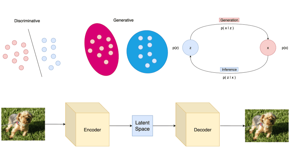
Machine Learning models are often categorized into discriminative and generative models. This distinction arises from the probabilistic formulation we use, to build and train those models.

Discriminative models learn the probability of a label $y$ based on a data point $x$ . In mathematical terms, this is denoted as $p( y | x)$ . In order to categorize a data point into a class, we need to learn a mapping between the data and the classes. This mapping can be described as a probability distribution. Each label will “compete” with the other ones for probability density over a specific data point.

Generative models, on the other hand, learn a probability distribution over the data points without external labels. Mathematically this is formulated as $p(x)$ . In this case, we have the data themselves “compete” for probability density.

Conditional Generative models are another category of models that try to learn the probability distribution of the data $x$ conditioned on the labels $y$ . As you can probably tell, this is denoted as $p(x|y)$ . Here we have again the data “compete” for density but for each possible label.

A thing that I want to clarify is this notion of competition. The probability density function $p$ is a normalized function, whose integral over all values is equal to 1.

\int_{X} p(x) dx =1

It is evident that each data point $x$ will only “acquire” a small piece of the density. As a result, each value $x$ will “compete with the other ones for a larger piece of the pie”.

Moreover, it is worth mentioning that the aforementioned model types are somewhat interconnected if we consider Bayes rule:

p(x | y) = \frac{p(y|x)}{p(y)} p(x)

This effectively tells us that we can build each type of model as a combination of the other types.

This time we will only focus on Generative models. We will derive the Variational Autoencoder model step by step through probabilities.

If you want to strengthen your skill in probability and statistics, he highly recommend the Introduction to Statistics. If you prefer a more techinical one, you should check Probabilistic Deep Learning with TensorFlow 2

Shall we begin?

Generative models

As we mentioned, the goal of generative models is to learn the probability density function $p(x)$ . This probability density effectively describes the behaviour of our training data and enables us to generate novel data by sampling from the distribution. Ideally , we want our model to learn a probability $p(x)$ density which will be identical to the density of our data $p_{data}(x)$ . Towards that goal, there are many different strategies.

The first class of models is able to actually compute the density function $p$ explicitly. This means that after training, we can feed a data point $x$ to the model and it will output the likelihood of the data point, which of course is the result of $p(x)$ . We refer to those models as explicit density models.

The second class, known as implicit density models, does not compute $p(x)$ . However, we are able to sample from the underlying distribution after the model is trained.

One can illustrate the generative model categories in a tree diagram:

Going even deeper, we can further extend this categorization.

Explicit density models can either compute exactly the density function or try to approximate it. Variational autoencoders fall in the latter category. We often refer to them as Latent Variable models.

Implicit density models are able to map the underlying distribution without computing it explicitly. They are mainly represented by Generative Adversarial Networks which have been presented in past articles. Feel free to check out our GANs in Computer Vision series.

Latent Variable models

Latent variable models aim to model the probability distribution with latent variables.

Latent variables are a transformation of the data points into a continuous lower-dimensional space.

Intuitively, the latent variables will describe or “explain” the data in a simpler way.

In a stricter mathematical form, data points $x$ that follow a probability distribution $p(x)$ , are mapped into latent variables $z$ that follow a distribution $p(z)$ .

Given that idea, we can now define five basic terms:

The prior distribution $p(z)$ that models the behaviour of the latent variables
The likelihood $p(x | z)$ that defines how to map latent variables to the data points
The joint distribution $p(x,z) =p(x|z)p(z)$ , which is the multiplication of the likelihood and the prior and essentially describes our model.
The marginal distribution $p(x)$ is the distribution of the original data and it is the ultimate goal of the model. The marginal distribution tells us how possible it is to generate a data point.
The posterior distribution $p(z|x)$ which describes the latent variables that can be produced by a specific data point

Notice that we don’t use any form of labels $y$ !

Finally, let’s define two more terms:

Generation refers to the process of computing the data point $x$ from the latent variable $z$ . In essence, we move from the latent space to the actual data distribution. Mathematically this is represented by the likelihood $p(x |z)$
Inference is the process of finding the latent variable $z$ from the data point $x$ and is formulated by the posterior distribution $p(z|x)$

It is evident that inference is the inverse of generation and vice versa.

Visually we can keep in mind the following diagram.

And here is the point where everything clicks together. If we assume that we somehow know the likelihood $p(x|z)$ , the posterior $p(z|x)$ , the marginal $p(x)$ , and the prior $p(z)$ we can do the following:

Generation

To generate a data point, we can sample $z$ from $p(z)$ and then sample the data point $x$ from $p(x|z)$

z \sim p(z)

x \sim p(x|z)

Inference

On the other hand, to infer a latent variable we sample $x$ from $p(x)$ and then sample $z$ from $p(z|x)$

x \sim p(x)

z \sim p(z|x)

The fundamental question of latent variable models: how do we find all those distributions?

And once again, I will remind you that the distributions are all interconnected due to the Bayes rule.

This is where Variational Autoencoders (VAE) come into play. To make sure that we can fully comprehend how they work, we first need to analyze all the building blocks and core ideas behind them.

If you are still with me, let’s continue.

Training a latent variable model with maximum likelihood

Maximum likelihood estimation is a well-established technique of estimating the parameters of a probability distribution so that the distribution fits the observed data. This is accomplished by maximizing a likelihood function.

A likelihood function measures the goodness of fit of a statistical model to a sample of data and it is formed from the joint probability distribution of the sample.

Mathematically we have:

\theta^{ML} = arg \max_{\theta} \sum_{i=1}^{N} log p_{\theta}(x_{i})

As you can tell, it is a standard optimization problem. It can’t be solved analytically so we use an iterative approach such as gradient descent. Once it’s solved, we can derive the model parameters $\theta$ which effectively model the desired probability distribution.

Nonetheless, in order to apply gradient descent, we need to calculate the gradient of the marginal log-likelihood function. Using simple calculus and the Bayes rule, we can prove that:

\nabla log p_{\theta}(x) = \int p_{\theta}(z |x) \nabla_{\theta} log p_{\theta}(x,z) dz

Did you find the underlying problem here? In order to compute the gradient, we need to have the posterior distribution $p(z|x)$ . Once again, we return to the problem of Inference.

Computing the posterior distribution - Solving the Inference problem

As mentioned before, we have two separate categories of models. Models with tractable and intractable inference.

In mathematics, problems are said to be tractable if they can be solved in terms of a closed-form expression.

In our case, most of the time it’s quite hard to have a tractable inference. We can construct models such as Linear-Gaussian models or invertible models (normalizing flows) but that often adds computational complexity and we will not cover them in this post.

In approximate inference models, on the other hand, we have an intractable problem but we try to approximate the inference. There are two common approaches when it comes to approximate inference:

Markov Chain Monte Carlo methods and
Variational Inference.

As you may have guessed, we will dive into the second one.

Variational Inference

Variational inference approximates the intractable posterior distribution with a tractable one, which is computed using an optimization problem.

So we want to approximate the actual $p_{\theta}( z | x)$ , with another distribution $q_{\phi}( z | x)$ called the variational posterior. We will extract the variational posterior by optimizing over a space of possible distributions with respect to the variational parameters $\phi$ .

By now, you may ask how the approximation problem is actually formulated? If you follow closely, you already know the answer. We will approximate the marginal log-likelihood function.

But there is a small difference. Because the marginal log-likelihood is intractable, we instead approximate a lower bound $L_{\theta,\phi}(x)$ of it, also known as variational lower bound. As a result, we maximize the lower bound with respect to both the model parameters $\theta$ and the variational parameters $\phi$ . It can be proved that the lower bound is:

L_{\theta,\phi}(x) = \textbf{E}_{q_{\phi}(z)} \left[ log \frac{p_{\theta}(x,z)}{q_{\phi}(z|x)} \right] \leq log p_{\theta}(x)

This is commonly known as the Evidence Lower Bound (ELBO) and is the most common variational lower bound.

E is used to denote the expected value or expectation. The expectation of a random variable X is a generalization of the weighted average of X and can be thought as the arithmetic mean of a large number of X.

If we extend the ELBO equation even further, we derive:

L_{\theta,\phi}(x) = log p_{\theta}(x) - \textbf{KL}(q_{\phi}(z|x) || p_{\theta}(z|x))

KL refers to Kullback–Leibler divergence and in simple terms is a measure of how different a probability distribution is from a second one.

Kullback–Leibler divergence is defined as :

\text{KL}(P\parallel Q)=\int _{-\infty }^{\infty }p(x)\log \left({\frac {p(x)}{q(x)}}\right)dx

The KL divergence is known as the variational gap. In our case, it expresses the difference between the true posterior and the variational posterior. It is essentially a measure of how good our approximation is. As we train our model, we maximize ELBO which in turn will increase $log p_{\theta}(x)$ and decrease the variational gap.

Amortized Variational Inference

With a closer look at the ELBO equation, we can see that the posterior distribution is different for each data point $x$ , which means that we need to learn different variational parameters $\phi$ for each data point. To overcome this issue, we introduce amortized inference.

In amortized variational inference, we train an external neural network to predict the variational parameters instead of optimizing ELBO per data point.

This network is called the Inference network in some papers. So from now on, $\phi$ parameters will refer to the inference network weights.

The main model and the inference network are trained simultaneously by maximizing ELBO with respect to both $\theta$ and $\phi$ . Once we train the inference network, we can compute the variational posterior for a new data point by simply feeding the data point to the network

Computing the gradient of ELBO

So we know that we need to maximize ELBO with respect to both the model and variational parameters. This means that we need to compute the gradients of:

L_{\theta,\phi}(x) = \textbf{E}_{q_{\phi}(z)} \left[ log \frac{p_{\theta}(x,z)}{q_{\phi}(z|x)} \right] \leq log p_{\theta}(x)

Let's start with model parameters. Although exact gradient calculation is possible, a much better approach is to use Monte Carlo sampling. In a few terms, this is equal to the following statement: We generate a handful of samples for the variational posterior and average them. That way we estimate the gradients instead of calculating them in a closed form.

\nabla_{\theta} L_{\theta,\phi}(x) = \frac{1}{K} \sum_{k=1}^{K} \nabla_{\theta} log p_{\theta}( x,z^k) \quad with \quad z^k \sim q_{\phi}(z|x)

When it comes to variational parameters, things are a little trickier because ELBO is an expectation with respect to $\phi$ . Luckily we can pull the Reparameterization trick from our sleeves.

Reparameterization trick

Intuitively we can think of reparameterization trick as follows:

Because we cannot compute the gradient of an expectation, we “move” the parameters of the probability distribution from the distribution space to the expectation space. In other words, we want to rewrite the expectation so that the distribution is independent of the parameter $\theta$ . Then we simply take the gradient as we did for the model parameters.

This abstract idea can be formulated as transforming a sample from a fixed, known distribution to a sample from $q_{\phi}(z)$ . If we consider the Gaussian distribution, we can express $z$ with respect to a fixed $\epsilon$ , where $\epsilon$ follows the normal distribution N(0,1)

z = \mu +\sigma \epsilon \quad with \quad \epsilon \sim N(0,1)

The epsilon term introduces the stochastic part and it is not involved in the training process.

In a fully stochastic operation, you cannot perform backpropagation. So, instead, we keep a fixed part stochastic with epsilon and train the mean and the standard deviation.

Therefore, we can now compute the gradient and run backpropagation of ELBO with respect to the variational parameters. The whole process can be depicted in the following image:

Source: Alexander Amini and Ava Soleimany, Deep Generative Modeling | MIT 6.S191, http://introtodeeplearning.com/

Variational Autoencoders

It’s finally time to put it all together and build the infamous Variational Autoencoder. I’m sure that your head is buzzing right now so let’s look on the practical side from now on.

For our main model, we will of course choose a Neural Network. This network will parameterize the variational posterior $q_{\phi}(z|x)$ (also known as the Decoder).

self.decoder = tf.keras.Sequential(
        [
            tf.keras.layers.InputLayer(input_shape=(latent_dim,)),
            tf.keras.layers.Dense(units=7*7*32, activation=tf.nn.relu),
            tf.keras.layers.Reshape(target_shape=(7, 7, 32)),
            tf.keras.layers.Conv2DTranspose(
                filters=64, kernel_size=3, strides=2, padding='same',
                activation='relu'),
            tf.keras.layers.Conv2DTranspose(
                filters=32, kernel_size=3, strides=2, padding='same',
                activation='relu'),
            # No activation
            tf.keras.layers.Conv2DTranspose(
                filters=1, kernel_size=3, strides=1, padding='same'),
        ]
    )

def decode(self, z, apply_sigmoid=False):
    logits = self.decoder(z)
    if apply_sigmoid:
      probs = tf.sigmoid(logits)
      return probs
    return logits

def sample(self, eps=None):
    if eps is None:
      eps = tf.random.normal(shape=(100, self.latent_dim))
    return self.decode(eps, apply_sigmoid=True)

We will train the model using amortized variational inference so we need another neural network as the Inference network (also known as the Encoder), which will parameterize the likelihood $p_{\theta}(x|z)$ .

self.encoder = tf.keras.Sequential(
        [
            tf.keras.layers.InputLayer(input_shape=(28, 28, 1)),
            tf.keras.layers.Conv2D(
                filters=32, kernel_size=3, strides=(2, 2), activation='relu'),
            tf.keras.layers.Conv2D(
                filters=64, kernel_size=3, strides=(2, 2), activation='relu'),
            tf.keras.layers.Flatten(),
            # No activation
            tf.keras.layers.Dense(latent_dim + latent_dim),
        ]
    )

def encode(self, x):
    mean, logvar = tf.split(self.encoder(x), num_or_size_splits=2, axis=1)
    return mean, logvar

In order to generate samples from the Encoder and pass them to the Decoder, we also need to utilize the reparameterization trick. Don’t forget that we need to be able to run the backward pass during training.

def reparameterize(self, mean, logvar):
    eps = tf.random.normal(shape=mean.shape)
    return eps * tf.exp(logvar * .5) + mean

Note that we use Gaussians, so the decoder will output the mean and the variance of the likelihood.

But can we arbitrarily assume that the posterior and the likelihood will be Gaussian?

As a matter of fact, we can if we assume that the prior distribution $p(z)$ is a standard normal $N(0,1)$ . Of course, there are research approaches that use different distributions but it’s out of the scope of this article.

The two networks are trained jointly by maximizing the ELBO which, in the VAE case, it is written as:

L_{\theta,\phi}(x) = \textbf{E}_{q_{\phi}(z|x)} [ log p_{\theta}(x|z) ] - \textbf{KL}(q_{\phi}(z |x) || p_{\theta}(z))

Analysis of loss terms

The first term controls how well the VAE reconstructs a data point $x$ from a sample $z$ of the variational posterior and it is known as negative reconstruction error. The second term controls how close the variational posterior is to the prior.

def compute_loss(model, x):
    mean, logvar = model.encode(x)
    z = model.reparameterize(mean, logvar)
    x_logit = model.decode(z)

    marginal_likelihood = tf.reduce_sum(x * tf.log(x_logit) + (1-x) * tf.log(1-x_logit),1)
    KL_divergence = 0.5* tf.reduce_sum (tf.square(mean) + tf.square(logvar) -tf.log(1e-8   + tf.square(logvar)) -1,1

    ELBO = tf.reduce_mean(marginal_likelihood) - tf.reduce_mean(KL_divergence)
    return - ELBO

As you can see from the code, during training:

We pass a datapoint to the encoder which will output the mean and the log-variance of the approximate posterior
We apply the reparameterization trick
We passed the reparameterized samples to the decoder, which will output the likelihood.
We compute the ELBO and backpropagate the gradients

To generate a new data point:

We sample a set of latent vectors from the Normal prior distribution
We obtain the latent variables from the encoder
The decoder will transform the latent variable of the sample to a new data point

sample = tf.random.normal(
    shape=[num_examples_to_generate, latent_dim])

def generate(model, epoch, test_sample):
  mean, logvar = model.encode(test_sample)
  z = model.reparameterize(mean, logvar)
  predictions = model.sample(z)

And that’s all. I hope that now, the mathematics described in the beginning of the article make some sense. For the full source code, please refer to the original Tensorflow implementation of VAE, which has been slightly modified for the purpose of this article.

Conclusion

In this article, we analyzed latent variable models and concluded by formulating a variational autoencoder approach. Due to their probabilistic nature, one will need a solid background on probabilities to get a good understanding of them. If you want to follow up on developing a VAE from scratch with Pytorch, please check our past article on Autoencoders.

References

[1] Kingma D, Welling M, (2013), Auto-Encoding Variational Bayes, arXiv:1312.6114

[2] Goodfellow I., Bengio Y., Courville A. ,(2016), Deep Learning, MIT Press

[3] Johnson J., (2020), EECS 498-007 / 598-005 Deep Learning for Computer Vision, University of Michigan

[4] Mnih A., (2020), DeepMind x UCL, Deep Learning Lectures , 11/12 , Modern Latent Variable Models

[5] Lilian W, (2018), From Autoencoder to Beta-VAE, lilianweng.github.io/lil-log

[6] Jordan J., (2018), Variational Autoencoders, jeremyjordan.me

[7] Rocca J, (2019), Understanding Variational Autoencoders (VAEs), towardsdatascience.com

[8] Hinton G. E, Salakhutdinov R. R., (2006), Reducing the Dimensionality of Data with Neural Networks, Science: Vol. 313, Issue 5786, pp. 504-507

[9] Blei D., Kucukelbir A., McAuliffe J., (2018), Variational Inference: A Review for Statisticians, arXiv:1601.00670v9

* Disclosure: Please note that some of the links above might be affiliate links, and at no additional cost to you, we will earn a commission if you decide to make a purchase after clicking through.