For a comprehensive list of all the papers and articles of this series check our Git repo
For a hands-on course we highly recommend coursera's brand-new GAN specialization
An important lesson from my journey in GANs is that you cannot start to learn deep learning from GANs. There is a tremendous set of background knowledge to understand each design choice. Each paper has its own creativity that derives from a general understanding of how deep learning really works. Proposing general solutions in generative learning is extremely tough. But when you start to focus on the specific tasks, creativity has no ceiling in the game of designing a GAN. This is one of the reasons that we chose to focus on computer vision. After a bunch of reviews, you start to understand that the top papers we include start to make sense. It is indeed like a puzzle.
So, let’s try to solve it!
In the previous post, we discussed 2K image-to-image translation, video to video synthesis, and large-scale class-conditional image generation. Namely, pix2pixHD, vid-to-vid, and BigGAN. In this part, we will start with unconditional image generation in ImageNet, exploiting the recent advancements in self-supervised learning. Finally, we will focus on style incorporation via adaptive instance normalization. To do so, we will revisit concepts of in-layer normalization that will be proven quite useful in our understanding of GANs.
Self-Supervised GANs via Auxiliary Rotation Loss (2018)
We have already discussed a lot about class-conditional GANs (BigGAN) as well as image-conditioned ones (pix2pixHD), in the previous post. These methods have achieved high quality in large resolutions, specifically 512x512 and 2048x1024, respectively. Nevertheless, we did not discuss what problems one may face when he tries to scale GANs in an unconditional setup.
This is one of the first works that bring ideas from the field of self-supervised learning into generative adversarial learning on large scales. Moreover, it is revolutionary in terms of introducing the notion of forgetting in GANs, as well as a method to encounter it. Unlabeled data are abundant compared to human-annotated datasets that are fairly limited. Therefore, it is a direction that we would like to explore.
Before we start, let’s clarify one thing that may seem vague in the beginning: the role of self-supervision targets the discriminator in order to learn meaningful feature representations. Through adversarial training, the generator is also affected by the injection of self-supervised guidance. Now, let us start by first understanding the notion of self-supervision.
1. What is self-supervised learning?
In general, GANs are considered a form of unsupervised learning. But why? The reason is basically that all data have the label “real”, while the generated ones have the label “fake” (at least for the training of D).
Unsupervised means we have no information on the data so basically we cannot simply create a loss function and backpropagate. In other words, with GANs we do this via labeling all the training data as real. So, we cast the problem as binary classification: real VS fake.
Unsupervised data exists in large quantities. What if we could produce “accurate and cheap labels” from the data itself? Since we are focusing on computer vision, we refer to generating labels from the images or videos. In other words, we set learning objectives properly (in unlabeled data) so as to get supervision from the data itself. This is what self-supervised learning is all about!
With self-supervised learning, one can guide the training process via an invented supervised loss function. It is worth noting that we don’t actually care about the results of the task that we design. Instead, our aim is to learn meaningful intermediate representations. It is assumed that the learned representation has memorized relative semantic or structural information to the task that we want to solve.
In simple terms, self-supervised refers to producing fairly accurate and computationally cheap labels.
Accurate refers to the fact that we want to be almost sure that the label is correct. Some may wonder why we don't use well-trained models to predict some sort of downstream label from the image. This can indeed be a good choice given that the model can achieve very good accuracy. However, this is not always the case. Some successful large-scale examples can be found in Xie et. al. 2019.
Cheap refers to the fact that we don't use humans to annotate. It is usually the case that the label is generated from the image/video. In general, any transformation is acceptable. The big question is how can you choose the self-supervised task? This is where it gets really creative. In essence, we are strongly based on the assumption that the task that we choose provides guidance for learned representations that are meaningful for our desired task, which in our case is unconditional image generation. Finally, keep in mind that we usually refer to a self-supervised task as a pretext or proxy task.
Self-supervised rotation baseline
Let’s start by inspecting the baseline purely self-supervised approach by Gidaris et al. In our case, the authors chose to apply rotation in the images of certain degrees {0, 90, 180, 270}, while D tries to find which rotation has been applied to the real image. For each image, 4 different rotations are applied as illustrated in the image below.
 Image is taken from the original work of Gidaris et al. ICLR 2018
In this way, the model (D in our case) is guided to learn semantic feature learning content via recognizing rotations.
GAN instability from forgetting
During training GANs, instability may arise from the fact that the generator and discriminator
learn in a non-stationary environment. Let’s see this through the math:
In the well-known equation, you probably observed that PG changes during training. It is the generated distribution of hallucinated images. This is where the term non-stationary training comes from. It is known that, in non-stationary online environments such as GANs, models forget previous tasks [Kirkpatrick et al. 2017]. Online refers to the alternating gradient descent training of G and D.
Let’s see an interesting experiment to clarify this concept.
The authors trained the same model with and without self-supervision in ImageNet without labels (unconditional setup). As you see in the depicted figure after 500k iterations performance decreases. This performance drop of the unconditional GAN indicates that information about the images (in this case the class label) is acquired and later forgotten. This is what we call forgetting and it is related to training instability. By adding the right self-supervised task, information forgetting is restricted.
 Figure: Analyzing and understanding forgetting of D in unconditional setup, taken from the original work.
Someone may wonder: how is this accuracy acquired? Well, for each of the 100k iterations, they train offline a logistic regression classifier on the last feature maps. So they evaluate the performance by classifying the 1000 ImageNet classes (or 10 classes in CIFAR10). As a matter of fact, ImageNet contains 1.3M images so we are basically seeing that this phenomenon is pretty intense.
Proposed solution: Collaborative Adversarial Training
As explained, G does not involve any rotation in its architectures. The hallucinated images are only rotated to be fed in D. Apart from the adversarial zero-sum game, G and D collaborate in order to encounter the auxiliary rotation task. Interestingly, D is trained to detect rotations based only on true data. Even though hallucinate images are rotated D parameters are not updated. Since G is encouraged to generate images that look like the real ones, it tends to produce rotation-detectable images. Consequently, D and G are collaborative with respect to the rotation task.
In more practical terms, the authors used a single D with two final layers for rotations detection and for distribution discrimination(real vs fake), QD, and PD, respectively. Mathematically, this can be expressed as:
In this equation, V is the well known adversarial criterion, R is the set of possible rotations, r is the chosen rotation, x superscript r is the rotated real image, and α, β are the hyperparameters. Note that, in G loss the rotation detection of the real images is indicated. In this way, G learns to generate images, whose representations in the feature space of D allows detecting rotations. However, convergence to the real data distribution is not guaranteed by this additional constraint. That’s why, α starts from a positive value around 0.2 and is slowly reduced to zero, while β is simply set to 1.
Results and discussion
In the experiments, the authors used ResNet architectures for G and D, similar to Miyato et al., as well as the proposed hinge loss to discriminate the real images. In addition, they used a batch size of 64, which is basically 16 images rotated in the set {0, 90, 180,270} for the smaller datasets like CIFAR-10. For the experiments in ImageNet, they trained the model on 128 cores of TPU, using a batch size of 2048, with resized images of 128x128 resolution. Let’s see some images:
 Results of randomly generated images trained on ImageNet in 128x128 resolution, as reported in the original work.
The core finding is that, under the same training conditions, the self-supervised GAN closes the gap in natural image synthesis between unconditional and conditional models. In other words, self-supervised GANs can match equivalent conditional GANs on the task of image synthesis, without having access to labeled data.
One reason to explain the worst performance in the baseline model (named Cond-GAN) is that it probably overfits the training data. One could inspect the representation performance of Cond-GAN on the training data for this. Authors claim to found a generalization gap, which possibly indicates overfitting.
In the opposite direction, when they remove the adversarial loss leaving just the rotation loss, the representation quality substantially decreases. This study indicates that the adversarial and rotation losses probably complement each other, both in terms of quantitative and qualitative results. Finally, we conclude by highlighting that the representation quality and image quality are related. This work proves with undeniable evidence that the idea of self-supervised-GANs is not trivial, as the proposed model does learn powerful image representations.
StyleGAN (A Style-Based Generator Architecture for Generative Adversarial Networks 2018)
Building on our understanding of GANs, instead of just generating images, we will now be able to control their style! How cool is that? But, wait a minute. We already saw in part 1 (InfoGAN) that controlling image generations is dependent on disentangled representations. Let’s see how one can design such a network step by step.
This work is heavily dependent on Progressive GANs, Adaptive Instance Normalization(AdaIN), and style transfer. We have already covered Progressive GANs in the previous part, so let’s dive into the rest of them before we focus on the understanding of this work.
Understanding feature space normalization and style transfer
The human visual system is strongly attuned to image statistics. It is known that spatially invariant statistics such as channel-wise mean and variance reliably encode the style of an image. Meanwhile, spatially varying features encode a specific instance.
Batch normalization
Batch Normalization (BN) normalizes the mean and standard deviation for each individual feature channel. Mean and standard deviation of image features are first-order statistics that relate to global characteristics that are visually appealing such as style. Taking into consideration all the image features we somehowmix their global characteristics. This strategy is actually very good when we want our representation to share these characteristics, such as in downstream tasks (image classifications). Mathematically, this can be expressed as:
N is the number of image batch H the height and W the width. The Greek letter μ() refers to mean and the Greek letter σ() refers to standard deviation. Similarly, γ and β correspond to the trainable parameters that result in the linear/affine transformation, which is different for all channels. Specifically γ,β are vectors with the channel dimensionality. The batch features are x with a shape of [N, C, H, W], where the index c denotes the per-channel mean. Notably, the spatial dimensions, as well as the image batch, are averaged. This way, we concentrate our features in a compact space, which is usually beneficial.
However, in terms of style and global characteristics, all individual channels share the shame learned characteristics, namely γ,β. Therefore, BN can be intuitively understood as normalizing a batch of images to be centered around a single style. Still, the convolutional layers are able to learn some intra-batch style differences. As such, every single sample may still have different styles. This, for example, was undesirable if you want to transfer all images to the same shared style (i.e. Van Gogh style).
But what if we don't mix the feature batch characteristics?
Instance normalization
Different from the BN layer, Instance Normalization (IN) is computed only across the features spatial dimensions, but again independently for each channel (and each sample). Literally, we just remove the sum over N in the previous equation. Surprisingly, it is experimentally validated that the affine parameters in IN can completely change the style of the output image. As opposed to BN, IN can normalize the style of each individual sample to a target style (modeled by γ and β). For this reason, training a model to transfer to a specific style is easier. Because the rest of the network can focus its learning capacity on content manipulation and local details while discarding the original global ones (i.e. style information).
In this manner, by introducing a set that consists of multiple γ, one can design a network to model a plethora of finite styles, which is exactly the case of conditional instance normalization.
Adaptive Instance Normalization (AdaIN)
The idea of style transfer of another image starts to become natural. What if γ, β is injected from the feature statistics of another image? In this way, we will be able to model any arbitrary style by just giving our desired feature image mean as β and variance as γ. AdaIN does exactly that: it receives an input x(content) and a style input y, and simply aligns the channel-wise mean and variance of x to match those of y. Mathematically:
That's all! So what can we do with just a single layer with this minor modification? Let us see!
 Architecture and results using AdaIN. Borrowed from the original work.
In the upper part, you see a simple encoder-decoder network architecture with an extra layer of AdaIN for style alignment. In the lower part, you see some results of this amazing idea! To summarize, AdaIN performs style transfer (in the feature space) by aligning the first-order statistics (μ and σ), at no additional cost in terms of complexity. If you want to play around with this idea code is available here (official) and here (unofficial)
The style-based generator
Let’s go back to our original goal of understanding Style-GAN. Basically, Nvidia in this work totally nailed our understanding and design of the majority of the generators in GANs. Let’s see how.
In a common GAN generator, the sampled input latent space vector z is projected and reshaped, so it will be further processed by transpose convolutional or upsample with or without convolutions. Here, the latent vector is transformed by a series of fully connected layers, the so-called mapping network f! This results in another learned vector w, called intermediate latent space W. But why would somebody do that?
 The awesome idea of a style-based generator. Taken from the original Style-GAN paper
Mapping network f
The major reason for this choice is that the intermediate latent space W does not have to support sampling according to any fixed distribution. With continuous mapping, its sampling density is induced. This mapping f “unwraps” the space of W, so it implicitly enforces a sort of disentangled representation. This means that the factors of variation become more linear. The authors argue that it will be easier to generate realistic images based on a disentangled representation compared to entangled ones. With this totally unsupervised trick, we at least expect W to be less entangled than Z space. Let’s move onto the depicted A in the figure.
A block: the style features
Then, the vector w is split by half, resulting in two learned sub-vectors (ys and yb in the paper) that correspond to the style feature statistics (affine transformation) of adaptive instance normalization (AdaIN) operations. The latter is placed after each convolutional layer of the synthesis network. Each such block will be used to model a different style variation in the same image.
B block: noise
Furthermore, the authors provide G with explicit noise inputs, as a direct method to model stochastic details. B blocks are single-channel images consisting of uncorrelated Gaussian noise. They are fed as an additive noise image to each layer of the synthesis network. The single noise image is broadcasted to all feature maps.
Synthesis network g
The synthesis network g consists of blocks starting from 4x4 to 1024x1024 similarly to the baseline architecture of Progressive growing GANs. To move from one block to the next, the spatial dimension is doubled by bilinear up-sampling layers. Similarly in D, bilinear downsampling is performed. The blocks are incrementally added, based on the intuition that the network gradually learns low-level information first. In this way, the new blocks model finer details.
Now, let’s look inside the synthesis block. A fundamental difference is that the initial low dimensional input of the network g is a constant tensor of 4x4x512, instead of a projected and reshaped random sampling vector.
Except for the initial block, each layer starts with an upsampling layer to double spatial resolution. Then, a convolution block is added. After each convolution, a 2D per-pixel noise is added to model stochasticity. Finally, with the magic AdaIN layer, the learned intermediate latent space that corresponds to style is injected.
Style mixing and truncation tricks
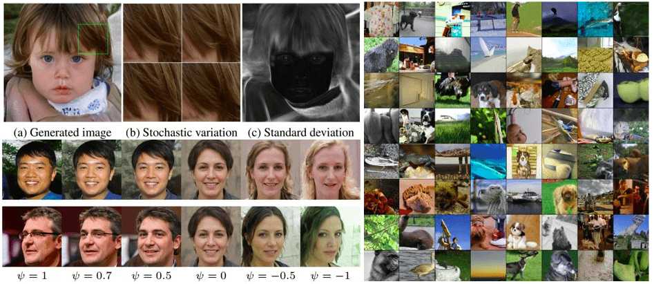
Instead of truncating the latent vector z as in BigGAN, the use it in the intermediate latent space W. This is implemented as: w’ = E(w) - ψ* ( w - E(w) ), where E(w)= E(f(z)). Ε denotes the expected value. The important parameter that controls sample quality is ψ. When it is closer to 0, we roughly get the sampled faces converging to the mean image of the dataset. Truncation in W space seems to work well as illustrated in the image below:
 Taken from the original Style-GAN paper
As perfectly described by the original paper: “It is interesting that various high-level attributes often flip between the opposites, including viewpoint, glasses, age, coloring, hair length, and often gender.”
Another trick that was introduced is the style mixing. Sampling 2 samples from the latent space Z they generate two intermediate latent vectors w1, w2 corresponding to two styles. w1 is applied before the crossover point and w2 after it. This probably is performed inside the block. This regularization trick prevents the network from assuming that adjacent styles are correlated. A percentage of generated images (usually 90%) use this trick and it is randomly applied to a different place in the network every time.
Looking through the design choices of the style-based generator
Each injected style and noise (blocks A and B) are localized in the network. This means that when modifying a specific subset of styles/noises, it is expected to affect only certain aspects of the image.
Style: Let’s see the reason for this localization, starting from style. We extensively saw that AdaIN operation first normalizes each channel to zero mean and unit variance. Then, it applies the style-based scales and biases. In this way, the feature statistics for the subsequent convolution operation are changed. Less literally, previous statistics/styles are discarded in the next AdaIN layer. Thus, each style controls only one convolution before being overridden by the next AdaIN operation.
Noise: In a conventional generator, the latent vector z is fed in the input of the network. This is considered sub-optimal as it consumes the generator's learning capacity. This is justified as the need of the network to invent a way to generate spatially-varying numbers from earlier activations.
By adding per-pixel noise after each convolution, it is experimentally validated that the effect of noise appears localized in the network. New noise is available for every layer, similar to BigGAN, and thus there is no motivation to generate the stochastic effects from previous activations.
Moreover, localized styles globally affect the entire image. Since AdaIN is applied to feature maps, global style/effects such as pose and lighting can be controlled. More importantly, they are coherent, because style is a global characteristic. In parallel, the noise is added independently to each pixel and is thus ideally suited for controlling small and local stochastic variations. As a consequence, the global (style) and local (noise) are learned without additional and explicit guidance to the network.
All the above can be illustrated below:
 Taken from the original Style-GAN paper
On the left, we have the generated image. In the middle, 4 different noises applied to a selected sub-region. The standard deviation of a big set of samples with different noise can be observed on the right.
Quantifying disentanglement of spaces
The awesomeness arises by the fact that they were also able to quantify the disentanglement of spaces for the first time! Because if you can't count it, it doesn't exist! To this end, they introduce two new ways of quantifying the disentanglement of spaces.
Perceptual path length
In case you don't feel comfortable with entangled and disentangled representations you can revisit InfoGAN. In very simple terms, entangled is mixed and disentangled related to encoded but separable in some way. I like to refer to disentangled representations as a kind of decoded information of a lower dimensionality of the data.
Let us suppose that we have two latent space vectors and we would like to interpolate between them? How could we possibly identify that the “walking of the latent space” corresponds in an entangled or disentangled representation? Intuitively, a less-sharp latent space should result in a perceptually smooth transition as observed in the image.
Interpolation of latent-space vectors can tell us a lot. For instance, non-linear, non-smooth, and sharp changes in the image may appear. How would you call such a representation? As an example, features that are absent in either endpoint can appear in the middle of a linear interpolation path. This is a sign of a messy world, namely entangled representation.
The quantification comes in terms of a small step ε in the latent space. If we subdivide a latent space interpolation path into small segments, we can measure a distance. The latter is measured between two steps, specifically, t, where t in [0,1] and t+ε. However, it is meaningful to measure the distance based on the generated images. So, one can sum the distances from all the steps to walk across two random samples of latent space z1 and z2. Note that the distance is measured in the image space. Actually, in this work, they measure the pairwise distance between two VGG network embeddings. Mathematically this can be described as (slerp denotes spherical interpolation):
Interestingly, they found that by adding noise, the path length (average distance) is roughly halved while mixing styles is a little bit increased (+10%). Furthermore, this measurement proves that the 8-layer fully connected architecture clearly produces an intermediate latent space W, which is more disentangled than Z.
Linear separability
Let’s see how this works.
We start by generating 200K images with z ∼ P (z) and classify them using an auxiliary classification network with label Y.
We keep 50% of samples with the highest confidence score. This results in 100k high-score auto-labeled (Y) latent-space vectors z for progressive GAN and w for the Style-GAN.
We fit a linear SVM to predict the label X based only on the latent-space point ( z and w for the Style-GAN) and classify the points by this plane.
We compute the conditional entropy H(Y | X) where X represents the classes predicted by the SVM and Y are the classes determined by the classifier.
We calculate the separability score as exp( Σ (H(Y| X) ) ), summing for all the given attributes of the dataset. We basically fit a model for each attribute. Note that the CelebA dataset contains 40 attributes such as gender info.
Quantitative results can be observed in the following table:
 Taken from the original Style-GAN paper
In essence, the conditional entropy H tells how much additional information is required to determine the true class of a sample, given the SVM label X. An ideal linear SVM would result in knowing Y with full certainty resulting in entropy of 0. A high value for the entropy would suggest high uncertainty, so the label based on a linear SVM model is not informative at all. Less literally,the lower the entropy H, the better.
As a final note, you can reevaluate your understanding by watching the official accompanying video.
Conclusion
If you followed our GANs in computer vision article series, you would probably get to the point that GANs are unstoppable. Personally speaking, GANs engineering and their solutions never cease to amaze me. In this article, we highlight the importance of self-supervision and the interesting directions that appear. Then, we see some exciting and careful generator design to inject the style of a reference image via adaptive instance normalization. Style-GAN is definitely one of the most revolutionary works in the field. Finally, we highlighted the proposed metrics for linear separability, which makes us dive into more and more advanced concepts in this series.
I really do hope that our co-learners are able to keep up with this. A great deal of work from our team is dedicated to making this series simple and precise. As always, we focus on intuition and we believe that you are not discouraged to start experimenting with GANs. If you would like to start experimenting with a bunch of models to reproduce the state-of-the-art results, you should definitely check this open-source library in Tensorflow or this one in Pytorch.
That being said, get ready for the next part.
We will be back for more!
For a hands-on video course we highly recommend coursera's brand-new GAN specialization.However, if you prefer a book with curated content so as to start building your own fancy GANs, start from the "GANs in Action" book! Use the discount code aisummer35 to get an exclusive 35% discount from your favorite AI blog.
Cited as:
@article{adaloglou2020gans,title = "GANs in computer vision",author = "Adaloglou, Nikolas and Karagianakos, Sergios",journal = "https://theaisummer.com/",year = "2020",url = "https://theaisummer.com/gan-computer-vision-style-gan/"}
References
- Karras, T., Laine, S., & Aila, T. (2019). A style-based generator architecture for generative adversarial networks. In Proceedings of the IEEE Conference on Computer Vision and Pattern Recognition (pp. 4401-4410).
- Ioffe, S., & Szegedy, C. (2015). Batch normalization: Accelerating deep network training by reducing internal covariate shift. arXiv preprint arXiv:1502.03167.
- Ulyanov, D., Vedaldi, A., & Lempitsky, V. (2016). Instance normalization: The missing ingredient for fast stylization. arXiv preprint arXiv:1607.08022.
- Xie, Q., Hovy, E., Luong, M. T., & Le, Q. V. (2019). Self-training with Noisy Student improves ImageNet classification. arXiv preprint arXiv:1911.04252.
- Chen, T., Zhai, X., Ritter, M., Lucic, M., & Houlsby, N. (2019). Self-supervised gans via auxiliary rotation loss. In Proceedings of the IEEE Conference on Computer Vision and Pattern Recognition (pp. 12154-12163).
- Kirkpatrick, J., Pascanu, R., Rabinowitz, N., Veness, J., Desjardins, G., Rusu, A. A., ... & Hassabis, D. (2017). Overcoming catastrophic forgetting in neural networks. Proceedings of the national academy of sciences, 114(13), 3521-3526.
- Miyato, T., Kataoka, T., Koyama, M., & Yoshida, Y. (2018). Spectral normalization for generative adversarial networks. arXiv preprint arXiv:1802.05957.

* Disclosure: Please note that some of the links above might be affiliate links, and at no additional cost to you, we will earn a commission if you decide to make a purchase after clicking through.