- For a comprehensive list of all the papers and articles of this series check our Git repo
We have seen so many important works in generative learning for computer vision. GANs dominate deep learning tasks such as image generation and image translation. In the previous post, we reached the point of understanding the unpaired image-to-image translation. We produced high-quality images from segmentations maps and vice versa. Nevertheless, there are some really important concepts that you have to understand before you implement your own super cool deep GAN model. In this part, we will take a look at some foundational works. We will see the most common gan distance function and why it works. Then, we will perceive the training of GANs as an attempt to find the equilibrium of a two-player game. Finally, we will see a revolutionary work of incremental training that enabled for the first time realistic megapixel image resolution.
The studies that we will explore mainly tackle mode collapse and training instabilities. Someone who has never trained a GAN would easily argue that we always refer to these two axes. In real life, training a large-scale GAN for a new problem can be a nightmare. That’s why we want to provide the best and most cited bibliography to encounter them.
It is nearly impossible to succeed in training novel GANs in new problems if you start reading and implementing the most recent approaches. Actually, it is like winning the lottery. By the time you move away from the most common datasets (CIFAR, MNIST, CELEBA) you are in chaos. Our review series aims to help exactly these people that like us, are super ambitious but don’t want to spend all of their time reading all the bibliography of the field. We hope our posts will bring you multiple ideas and novel intuitions and perspectives to tackle your own problems.
Wasserstein GAN (2017)
It is usually the case that you try to visually understand the learning curves as debugging so as to guess the hyperparameters that might work better. But the GAN training is so unstable that this process is often a waste of time. This adorable work is one of the first to provide extensive theoretical justifications for the GAN training scheme. Interestingly, they found patterns between all the existing distances between distributions.
Core idea
The core idea is to effectively measure how close is the model distribution to the real distribution. Because the choice of how you measure the distance directly impacts on the convergence of the model. As we now know, GANs can represent distributions from low dimensional manifolds(noise z). Intuitively, the weaker this distance, the easier it is to define a mapping from the parameter space (θ-space) to the probability space since it’s proven to be easier for the distributions to converge. We have a reason to require this continuous mapping. Mainly, because it is possible to define a continuous function that satisfies this continuous mapping that gives as the desired probability space or generated samples.
For this reason, this work introduces a new distance called Wasserstein-GAN. It is an approximation of the Earth Mover (EM) distance, which theoretically shows that it can gradually optimize the training of GAN. Surprisingly, without the need to balance D and G during training, as well as it does not require a specific design of the network architectures. In this way, mode collapse which inherently exists in GANs is reduced.
Understanding Wasserstein distance
Before we dive into the proposed loss, let us see some math. As perfectly described in wiki, the supremum(sup) of a subset S of a partially ordered set T is the least element in T that is greater than or equal to all elements of S. Consequently, the supremum is also referred to as the least upper bound. I personally refer to it as the maximum of the subset of all possible combinations that can be found in T.
Now, let’s bring this concept in our GAN terminology. T is all the possible pair functions approximations f that we can get from G and D. S will be the subset of those functions that we will constrain to make training better (some sort of regularization). Ordering will come naturally from the computed loss function. Based on the above we can finally see the Wasserstein loss function that measures the distance between the two distributions Pr and Pθ.
The strict mathematical constraint is called K-Lipschitz functions to get the subset S. But you don’t need to know more math if it is extensively proven. But how can we introduce this constraint?
One way to deal with this is to roughly approximate this constraint is by training a neural network with its weights lying in a compact space. In order to achieve that the easiest thing to do is to just clamp the weights to a fixed range. That’s it, weight clipping works as we want to! Therefore, after each gradient update, we clip w range to [−0.01, 0.01]. That way, we significantly enforce the Lipschitz constraint. Simple but I can assure you it works!
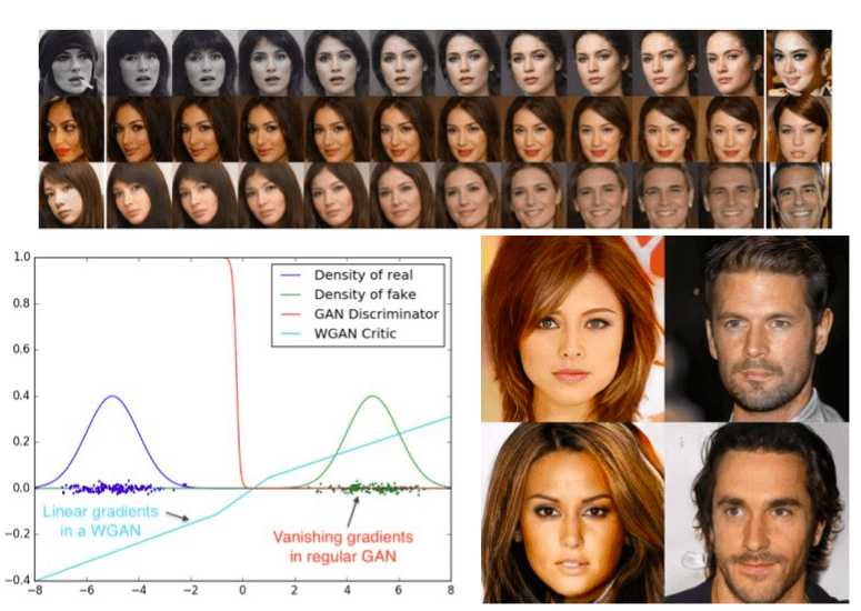
In fact, with this distance-loss function, which is, of course, continuous and differentiable, we can now train D with the proposed criterion till optimality, while other distances saturate. Saturation means that the discriminator has zero loss and the generated samples are only in some cases meaningful. So now, saturation (that naturally leads to mode collapse) is alleviated and we can train with more linear-style gradients for all the range of training. Let’s see an example to clarify this:
 Taken from WGAN. WGAN criterion provides clean gradients on all parts of the space.
To see all the previous math in practice, we provide the WGAN coding scheme in Pytorch. You can directly modify your project to include this loss criterion. Usually, it’s better to see it in real code. It’s important to mention that to save the subset and take the upper bound it means that we have to take a lot of pairs. That’s why you see that we train the generator every couple of times so that the discriminator get’s updates. In this way, we have the set to define the supremum. Notice that in order to approach the supremum we could also make a lot of steps for G before upgrading D.
import torchdef WGAN_train_step(optimizer_D, optimizer_G, generator, discriminator, real_imgs, clip_value, iteration, n_critic = 5):batch = real_imgs.size(0)# Train Discriminatoroptimizer_D.zero_grad()# Sample noise for dim=100z = torch.rand(batch, 100)# Generate a batch of imagesfake_imgs = generator(z).detach()# Adversarial lossloss_D = -torch.mean(discriminator(real_imgs)) + torch.mean(discriminator(fake_imgs))loss_D.backward()optimizer_D.step()# Clip weights of discriminatorfor p in discriminator.parameters():p.data.clamp_(-clip_value, clip_value)# Train the generator every couple of iterationsif iteration % n_critic == 0:optimizer_G.zero_grad()# Generate a batch of imagesz = torch.rand(batch, 100)gen_imgs = generator(z)# Adversarial lossloss_G = -torch.mean(discriminator(gen_imgs))loss_G.backward()optimizer_G.step()
In a later work, it was proved that even though this idea is solid, weight clipping is a terrible way to enforce the desired constraint. Another way to enforce the functions to be K-Lipschitz is the gradient penalty. The key idea is the same: to keep the weight in a compact space. However, they do it by constraining the gradient norm of the critic’s output with respect to its input. We will not cover this paper, but for consistency and easy experimentation for our users, we provide the code as an improved alternative to vanilla wgan. The code clarifies the required modifications to implement gradient loss on your problem.
import torchfrom torch.autograd import Variablefrom torch import autograddef WGAN_GP_train_step(optimizer_D, optimizer_G, generator, discriminator, real_imgs, iteration, n_critic = 5):"""Keep in mind that for Adam optimizer the official paper sets β1 = 0, β2 = 0.9betas = ( 0, 0.9)"""optimizer_D.zero_grad()# Sample noise for dim=100batch = real_imgs.size(0)z = torch.rand(batch, 100)# Generate a batch of fake imagesfake_imgs = generator(z).detach()# Find penalty between real and fake imagesgrad_penalty = gradient_penalty(discriminator, real_imgs, fake_imgs)# Adversarial loss + penaltyloss_D = -torch.mean(discriminator(real_imgs)) + torch.mean(discriminator(fake_imgs)) + grad_penaltyloss_D.backward()optimizer_D.step()# Train the generator every couple of iterationsif iteration % n_critic == 0:optimizer_G.zero_grad()# Generate a batch of imagesz = torch.rand(batch, 100)gen_imgs = generator(z)# Adversarial lossloss_G = -torch.mean(discriminator(gen_imgs))loss_G.backward()optimizer_G.step()def gradient_penalty(discriminator, real_imgs, fake_imgs, gamma=10):batch_size = real_imgs.size(0)epsilon = torch.rand(batch_size, 1, 1, 1)epsilon = epsilon.expand_as(real_imgs)interpolation = epsilon * real_imgs.data + (1 - epsilon) * fake_imgs.datainterpolation = Variable(interpolation, requires_grad=True)interpolation_logits = discriminator(interpolation)grad_outputs = torch.ones(interpolation_logits.size())gradients = autograd.grad(outputs=interpolation_logits,inputs=interpolation,grad_outputs=grad_outputs,create_graph=True,retain_graph=True)[0]gradients = gradients.view(batch_size, -1)gradients_norm = torch.sqrt(torch.sum(gradients ** 2, dim=1) + 1e-12)return torch.mean(gamma * ((gradients_norm - 1) ** 2))
Results and discussion
Following our brief description, we can now jump in some results. It is beautiful to see how a GAN learns during training, as illustrated below:
 Wasserstein loss criterion with DCGAN generator. The loss decreases quickly and stably, while sample quality increases. Taken from the original work.
This work is considered fundamental in the theoretical aspects of GANs and can be summarized as:
- Wasserstein criterion allows us to train D until optimality. When the criterion reaches the optimal value, it simply provides a loss to the generator that we can train as any other neural network.
- We no longer need to balance G and D capacity properly.
- Wasserstein loss leads to a higher quality of the gradients to train G.
- It is observed that WGANs are more robust than common GANs to the architectural choices for the generator and hyperparameter tuning
It is true that we have indeed gained improved stability of the optimization process. However, nothing comes at zero cost. WGAN training becomes unstable with momentum-based optimizers such as Adam, as well as with high learning rates. This is justified because the criterion loss is highly non-stationary, so momentum-based optimizers seemed to perform worse. That’s why they used RMSProp, which is known to perform well on non-stationary problems.
Finally, one intuitive way to understand this paper is to make an analogy with the gradients on the history of in-layer activation functions. Specifically, the gradients of sigmoid and tanh activations that disappeared in favor of ReLUs, because of the improved gradients in the whole range of values.
BEGAN (Boundary Equilibrium Generative Adversarial Networks 2017)
We often see that the discriminator progresses too fast at the beginning of training. Still, balancing the convergence of the discriminator and of the generator is an existing challenge.
This is the first work that is able to control the trade-off between image diversity and visual quality. With a simple model architecture and a standard training scheme the acquired high-resolution images.
To achieve this, the authors introduce a trick to balance the training of the generator and discriminator. The core idea of BEGAN is this newly enforced equilibrium that is combined along with described Wasserstein distance. To this end, they train an auto-encoder based discriminator. Interestingly, since D is now an auto-encoder, it produces images as output, instead of scalars. Let’s keep that in mind before we move on!
As we saw, matching the distribution of the errors instead of matching the distribution of the samples directly is more effective. A critical point is that this work is aiming to optimize the Wasserstein distance between auto-encoder loss distributions, not between sample distributions. An advantage of BEGAN is that it does not explicitly require the discriminator to be K-Lipschitz constrained. An autoencoder is usually trained with an L1 or L2 norm.
Formulation of the two-player game equilibrium
To express the problem in terms of game theory, an added equilibrium term to balance the discriminator and the generator is added. Suppose we can ideally generate indistinguishable samples. Then, the distribution of their errors should be the same, including their expected error, which is the one we measure after processing each batch. A perfectly balanced training will result in an equal expected value of L(x) and L(G(z)). However, this is never the case! Thus BEGAN decided to quantify the balance ration, defined as:
This quantity is modeled in the network as a hyperparameter. Therefore, the new training scheme involves two competing goals: a) auto-encode real images and b) discriminate
real from generated images. The γ term lets us balance these two goals. Lower values of γ lead to lower image diversity because the discriminator focuses more heavily on auto-encoding real images. But how is it possible to control this hyperparameter when the expected losses are varying?
Boundary Equilibrium GAN (BEGAN)
The answer is simple: we just have to introduce another variable kt that falls into the range [0, 1]. This variable will be designed to control the focus that is put on L(G(z)) during training.
It is initialized with k0 = 0 and λ_k is also defined as the proportional gain for k (used 0.001) in this study. This can be seen as a form of closed-loop feedback control, wherein kt is adjusted at each step to maintain the desired equilibrium for the chosen hyperparameter γ.
Note that, in the early training stages, G tends to generate easy-to-reconstruct data for D. Meanwhile, the real data distribution has not been learned accurately. Basically, L(x) > L(G(z)). As opposed to many GANs, BEGAN requires no pretraining and can be optimized with Adam. Finally, a global measure of convergence is derived, by using the equilibrium concept.
In essence, one can formulate the convergence process as finding a) the closest reconstruction L(x) and b) the lowest absolute value for the control algorithm || γ L(x)−L(G(z)) ||. Adding these two terms we can recognize when the network has converged.
Model architecture
The model architecture is quite plain. A major difference is the introduction of exponential linear units instead of ReLUs. They used an auto-encoder with both a deep encoder and a decoder. The hyper-parametrization intends to avoid typical GAN training tricks.
 BEGAN architecture is taken from the original work
A U-shaped architecture is used without skip connections. Down-sampling is implemented as a sub-sampling convolution with a kernel of 3 and a stride of 2. On the other hand, upsampling is done by the nearest neighbor interpolation. Between the encoder and the decoder, the
tensor of processed data is mapped via fully connected layers, not followed by any non-linearities.
Results and discussion
Some of the presented visual results can be seen in 128x128 interpolated images below:
 Interpolated 128x128 images generated by BEGAN
Notably, it is observed that variety increases with γ but so do artifacts (noise). As can be seen, the interpolations show good continuity. On the first row, the hair transitions and hairstyles are altered. It is also worth noting that some features disappear (cigarette) in the left image. The second and last rows show simple rotations. While the rotations are smooth, we can see that profile pictures are not captured perfectly.
As a final note, using the BEGAN equilibrium method, the network converges to
diverse and visually pleasing images. This remains true at 128x128 resolutions with trivial modifications. Training is stable, fast, and robust to small parameter changes.
But let us see what happens in really high resolutions!
Progressive GAN (Progressive Growing of GANs for Improved Quality, Stability, and Variation 2017)
The methods that we have described so far produce sharp images. However, they produce images only in relatively small resolutions and with limited variation. One of the reasons the resolution was kept low was training instability. If you have already deployed your own GAN models, you probably know that large resolutions demand smaller mini-batches, due to computational space complexity. In this manner, the problem of time complexity also rises, which means that you need days to train a GAN.
Incremental growing architectures
To address these problems authors progressively grow both the generator and discriminator, starting from low to high-resolution images. The intuition is that the newly added layers aim to capture higher-frequency details that correspond to high-resolution images, as the training progresses. But what makes this approach so good?
The answer is simple: instead of having to learn all scales simultaneously, the model first discovers large-scale (global) structure and then local fine-grained details. The incremental training nature aims in this direction. It is important to note that all layers remain trainable throughout the training process and the network architectures are symmetrical (mirror images). An illustration of the described architecture is depicted below:
 Taken from the original paper
However, mode collapse still exists, due to the unhealthy competition, which escalates the magnitude of the error signals in both G and D.
Introduction of a smooth layer between transition
The key innovation of this work is the smooth transition of the newly added layers to stabilize training. But what happens after each transition?
 Taken from the original paper
What is really happening is that the image resolution is doubled. Therefore, a new layer on G and D is added. This is where the magic happens. During the transition, the layers that operate on the higher resolution are utilized as a residual skip connection block, whose weight (α) increases linearly from 0 to 1. One means that the skip connection is discarded.
The depicted toRGB blocks represent a layer that projects and reshapes the 1-dimensional feature vectors to RGB colors. It can be regarded as the connecting layer that always brings the image in the right shape. In parallel, fromRGB does the reverse, whereas both use 1 × 1 convolutions. The real images are downscaled correspondingly to match the current dimension.
Interestingly, during a transition, authors interpolate between the two resolutions of the real images, to resemble GANs-like learning. Furthermore, with progressive-GAN most of iterations are performed at lower resolutions, resulting in 2 to 6 train speedup. Hence, this is the first work that reaches a megapixel resolution, namely 1024x1024.
Unlike downstream tasks that encounter covariance shift, GANs exhibit increasing error signal magnitudes and competition issues. To address them, they use normal distribution initialization and per-layer weight normalization by a scalar that is computed dynamically per batch. This is believed to make the model learn scale-invariance. To further constrain signal magnitudes, they also normalize the pixel-wise feature vector to unit length in the generator. This prevents the escalation of feature maps while not deteriorating the results significantly. The accompanying video may help in the understanding of the design choices. Official code is released in TensorFlow here.
Results and discussion
Results can be summarized as follows:
The improved convergence is explained by the gradually increasing network capacity. Intuitively, the existing layers learn the lower scale, so after the transition, the introduced layers are only tasked with refining the representations by increasingly smaller-scale effects.
The speedup from progressive growth increases as the output resolution grows. This enables for the first time the generation of crispy images of 1024x1024.
Even though it is really difficult to implement such an architecture and a lot of training details are missing (i.e. when to make a transition and why), it is still an incredible work that I personally adore.
 The official reported results in megapixel resolution taken from the original work
Conclusion
In this post, we encountered some of the most advanced training concepts that are used even today. The reason we focused on covering these important training aspects is to be able to present more advanced applications further on. If you want a more game-theoretical perspective of GANs we strongly advise you to watch Daskalakis talk. Finally, for our math lovers, there is a wonderful article here, that covers in more detail the transition to WGAN.
To conclude, we have already found a couple of ways to deal with mode collapse, large-scale datasets, and megapixel resolutions with incremental training. It is definitely a lot of progress. However, the best is yet to come!
In part 4, we will see the amazing advancements of GAN in computer vision starting from 2018!
For a hands-on video course we highly recommend coursera's brand-new GAN specialization.However, if you prefer a book with curated content so as to start building your own fancy GANs, start from the "GANs in Action" book! Use the discount code aisummer35 to get an exclusive 35% discount from your favorite AI blog.
Cited as:
@article{adaloglou2020gans,title = "GANs in computer vision",author = "Adaloglou, Nikolas and Karagiannakos, Sergios ",journal = "https://theaisummer.com/",year = "2020",url = "https://theaisummer.com/gan-computer-vision-incremental-training/"}
References
- Arjovsky, M., Chintala, S., & Bottou, L. (2017). Wasserstein gan. arXiv preprint arXiv:1701.07875.
- Berthelot, D., Schumm, T., & Metz, L. (2017). Began: Boundary equilibrium generative adversarial networks. arXiv preprint arXiv:1703.10717.
- Karras, T., Aila, T., Laine, S., & Lehtinen, J. (2017). Progressive growing of gans for improved quality, stability, and variation. arXiv preprint arXiv:1710.10196.
- Daskalakis, C., Ilyas, A., Syrgkanis, V., & Zeng, H. (2017). Training gans with optimism. arXiv preprint arXiv:1711.00141.
- Gulrajani, I., Ahmed, F., Arjovsky, M., Dumoulin, V., & Courville, A. C. (2017). Improved training of wasserstein gans. In Advances in neural information processing systems (pp. 5767-5777).

* Disclosure: Please note that some of the links above might be affiliate links, and at no additional cost to you, we will earn a commission if you decide to make a purchase after clicking through.