- For a comprehensive list of all the papers and articles of this series check our Git repo. However, if you prefer a book with curated content so as to start building your own fancy GANs, start from the "GANs in Action" book!
Whats is generative learning? What is a GAN? Why do we use it? What is the difference with autoencoders? What is the fundamental training algorithm of a GAN model? How can we make it learn meaningful representations? In what computer vision application can it be useful? How can one design one for her/his problem?
We will address all these questions and much much! In this review article series, we will focus on a plethora of GANs for computer vision applications. Specifically, we will slowly build upon the ideas and the principles that led to the evolution of generative adversarial networks (GAN). We will encounter different tasks such as conditional image generation, 3D object generation, video synthesis.
Let's start with reviewing our contents of the first part!
In general, data generation methods exist in a big variety of modern deep learning applications, from computer vision to natural language processing. At this point, we are able to produce nearly indistinguishable generative data by the human eye. Generative learning can be broadly divided into two main categories: a) Variational AutoEncoders (VAE) and b) generative adversarial networks (GAN).
Why not just autoencoders?
A lot of people are still wondering why researchers make things so difficult with GANs. Why don’t just use an autoencoder and minimize the mean squared error, having the target image to match the predicted one? The reason is that these models produce poor results (for image generation). Actually, just minimizing the distance produces blurry predictions because of the averaging. Remember the L1 or L2 loss is scalar, which is an average quantity of all the pixels. Intuitively, it is a similar concept as applying a smoothing filter that averages the pixel values based on the average. Second, it is impossible to produce diversity in such a way (like variational autoencoders). That’s why the attention of the research community adopted GAN models. Keep in mind that this is not a comparison but a differentiation of the GAN approach.
So, let’s start from the very beginning: what is adversarial learning anyway?
What is adversarial learning?
We have experimentally validated that deep learning models are highly vulnerable to attacks that are based on small modifications of the input to the model at test time. Suppose you have a trained classifier that correctly recognizes an object in an image with the correct label.
It’s possible to construct an adversarial example, which is a visually indistinguishable image. These adversarial images can be constructed by noise perturbation. However, the image is classified incorrectly. To address this problem, a common approach is to inject adversarial examples into the training set (adversarial training). Hence, the neural network’s robustness can be increased. This type of example can be generated by adding noise, by applying data augmentation techniques or by perturbating the image in the opposite direction of the gradient (to maximize loss instead of minimizing it). Nevertheless, these types of techniques are a little bit hand-crafted so there will always be a different perturbation that can be applied to fool our classifier. Now let’s think the other way around!
What if we are not interested in having a robust classifier, but rather we are interested in replacing the hand-crafted procedure of adversarial examples? In this way, we can let the network create different examples that are visually appealing. So, that’s exactly where the generative term comes into play. We focus on producing representative examples of the dataset instead of making the network more robust to perturbations! Let us use another network to do this work for us. How would you call a network that generates realistic examples similar to the training ones? Generator, of course!
Vanilla GAN (Generative Adversarial Networks 2014)
Generator
Since a generator is simply a neural network, we need to provide it with an input and decide what the output will be. In the simplest form, the input is random noise that is sampled from a distribution in a small range of real numbers. This is what we call latent or continuous space. However, since I use the word random it means that every time I sample from a random distribution, I will get a different vector sample. That’s what stochasticity is all about. Such input will provide us with a non-deterministic output. As a consequence, there is no limit to the number of samples we can generate! Stochasticity is also the reason why you see the symbol of expected value in the papers related to Generative Adversarial Learning (GAN). The output will be a generated image for image generation or something that we would like to generate. The main difference is that now we focus on generating representative examples of a specific distribution (i.e. dogs, paintings, street pictures, airplanes, etc.)
Now, what about the discriminator?
Discriminator
The discriminator is nothing more than the classifier. However, instead of classifying an image in the correct class, we focus on learning the distribution of the class (let’s say producing building images). Therefore, since the desired class is known, we want the classifier to quantify how representative the class is to the real class distribution. That’s why discriminators output a single probability, wherein 0 corresponds to the fake generated images and 1 to the real samples from our distribution.
An ideal generator would produce indistinguishable examples which means an output of 0.5. In terms of game theory, this adversary is called a 2-player minmax game. In game theory, a min-max game or Nash equilibrium is a mathematical representation of a non-cooperative game involving two players, in which each player is assumed to know the equilibrium strategies of the other player, and no player has anything to gain by changing only their own strategy.
Generator G attempts to produce fake examples that are close to the real distribution so as to fool Discriminator D, while D tries to decide the origin of the distribution. The core idea that rules GANs is based on the “indirect” training through D that is also getting updated dynamically.
The generative adversarial training scheme
Based on the above principles, the first GAN was introduced in 2014. It is important to understand the training process of generative learning. One key insight is the indirect training: this basically means that the generator is not trained to minimize the distance to a specific image, but just to fool the discriminator! This enables the model to learn in an unsupervised manner. Finally, pay attention that the ground truth when training the generator is 1 (like a real image) in the output, even though the examples are fake. This happens because our objective is just to fool D. The image below illustrates this process:
 An illustration of the generator training scheme
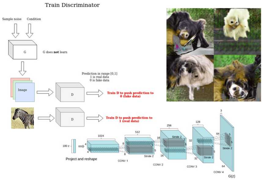
On the other hand, the discriminator uses the real image and the generated to distinguish them, pushing the prediction of the real image to 1(real) and the prediction of the generated image to 0 (fake). In this stage, notice that the Generator is not trained.
 An illustration of the discriminator training scheme
The authors of GAN proposed an architecture consisting of 4 fully-connected layers for both G and D. Of course, G outputs a 1-D vector of the image and D outputs a scalar in the range (0,1).
GAN training scheme in action
Representation gives us power over ideas. It is nice to understand the math before seeing the code. So, given discriminator D, generator G, vale function V the fundamental two-player minimax game can be defined as (M are the samples):
In practice, recalling the discete definition of the expected value, it looks like this:
In fact, the discriminator performs gradient ascend, while the generator performs gradient descent. This can be observed by inspecting the differences in the generator part of the above equations. Note that, D needs to access both real and fake data, while G has no access to the real images. Let’s see this beautiful yet amazing idea in practice in real python code:
import torchdef ones_target(size):'''For real data when training D, while for fake data when training GTensor containing ones, with shape = size'''return torch.ones(size, 1)def zeros_target(size):'''For data when training DTensor containing zeros, with shape = size'''return torch.zeros(size, 1)def train_discriminator(discriminator, optimizer, real_data, fake_data, loss):N = real_data.size(0)# Reset gradientsoptimizer.zero_grad()# Train on Real Dataprediction_real = discriminator(real_data)# Calculate error and backpropagatetarget_real = ones_target(N)error_real = loss(prediction_real, target_real)error_real.backward()# Train on Fake Dataprediction_fake = discriminator(fake_data)# Calculate error and backpropagatetarget_fake = zeros_target(N)error_fake = loss(prediction_fake, target_fake)error_fake.backward()# Update weights with gradientsoptimizer.step()return error_real + error_fake, prediction_real, prediction_fakedef train_generator(discriminator, optimizer, fake_data, loss):N = fake_data.size(0)# Reset the gradientsoptimizer.zero_grad()# Sample noise and generate fake dataprediction = discriminator(fake_data)# Calculate error and backpropagatetarget = ones_target(N)error = loss(prediction, target)error.backward()optimizer.step()return error
Now, let’s see some generated images. Image change corresponds to a different epoch.
 Generated Vanilla GAN images in Mnist
Mode collapse in GANs
In general, GANs are prone to the so-called mode collapse problem. The latter usually refers to the generator that fails to adequately represent the pixel-space of all the possible outputs. Instead, G selects just a few limited influential modes that correspond to noise images. In this way, D is able to distinguish real from fakes and the loss of the G gets highly unstable (due to exploding gradients). We will revisit mode collapse a lot of times in our series, thus it is crucial to grasp the basic principle.
Basically, G stucks in a parameter setting where it always emits the same point. After collapse has occurred, the discriminator learns that this single point comes from the generator, but gradient descent is unable to separate the identical outputs. As a result, the gradients of D push the single point produced by the generator around space forever.
Mode collapse may happen the other way around: If while training the discriminator gets stuck in a local minimum and he is not able to find the best strategy, then it's too easy for the generator to fool the current discriminator (in a couple of iterations).
Finally, I would explain mode collapse in simple terms as: the state of the 2-player game where one of the players gains an almost irreversible advantage, which makes it difficult to lose the game.
Conditional GAN (Conditional Generative Adversarial Nets 2014)
Conditional probability is a measure of the probability of an event occurring given that another event has occurred. In this work, the conditional version of GAN is introduced. Basically, conditional information can be utilized by simply feeding whatever "extra" data, such as image tags/labels, etc. By conditioning the model on auxiliary information, it is possible to guide the data generation process.
Based on the generation task, one can perform the conditioning by feeding information into both D and G, as additional input via concatenation. In other domains such as medical image generation, the condition may be demographic information (i.e. age, height) or semantic segmentation.
 Visual representation of conditioning a GAN taken from cGAN paper
DCGAN (Unsupervised Representation Learning with Deep Convolutional Generative Adversarial Networks 2015)
DCGAN was the first convolutional GAN. Deep Convolutional Generative Adversarial Nets (DCGAN) is a topologically constrained variant of GAN. In order to reduce the number of parameters per layer, as well as to make training faster and more stable the below principles were introduced:
Replace any pooling layers with strided convolutions in D. This can be justified because pooling is a fixed operation. In contrast, strided convolution can also be viewed as learning the pooling operation, which increases the model's expressiveness ability. The disadvantage is that it also increases the number of trainable parameters.
Use transpose convolutions in G. Because sampled noise is a 1D vector, it is usually projected and reshaped to a small 2D grid (i.e. 4x4), with an enormous amount of feature maps. That’s why G uses transpose convolutions to increase spatial dimensions (usually doubles them) and reduces the number of feature maps.
Use batch normalization in both G and D. Batch normalization stabilizes training and enables training with higher learning rate, based on the statistics of each batch in the layer.
Remove fully connected hidden layers for deeper architectures to reduce the number of training parameters and training time.
Use ReLU activation in G for all layers except for the output, which produces values in the image range [-1,1]
Use LeakyReLU activation in the discriminator for all layers. Both activation functions are nonlinear and enable the model to learn more complex representations.
D has fewer feature maps than the compared method (K-means). In general, for G and D, it is not clear which model should be more complex, because it is task-dependent. In this work, G has more trainable parameters than D. However, there is no theoretical justification behind this design choice.
 The unconditional generator of DCGAN
Results and discussion
Let’s observe the output of a DCGAN model in MNIST dataset, given a simple implementation
 Improved image quality with DCGAN
The output digits are more cripsy and contain less noise, using convolutional modules. If you want to observe mode collapse in practice you can try to train a DCGAN in CIFAR-10, using only one class:
 Observing mode collapse in DCGAN in CIFAR10, using one class
Basically, you start with noise. Then you have a fair representation with something that starts to look like the desired images. And then boom! The generator literally collapses it is the repeating square patterns. What happened? Mode collapse!.
To summarize, DCGAN is the standard convolutional baseline that most of the next architectures were based upon. It shows great improvement both in terms of visual quality (less blurriness) and training stability than the standard GAN. However, for larger scales like unconditional image generation of CIFAR-10 it has a lot of space for great engineering magic, as we will see. Finally, let’s look at the result of training DCGAN in the whole CIFAR-10 dataset with all classes.
 DCGAN in CIFAR10
Pretty fair, right?
Info GAN: Representation Learning by Information Maximizing Generative Adversarial Nets (2016)
We already talked about conditional variables of cGANs that are usually class labels or tags. However, there are two questions that are not answered:
a) how much of this information is passed into the generation process compared to noise, and
b) can a completely unsupervised condition that lies in a latent space help us "walk” in the generator space?
This work addresses these questions through disentangled representations and mutual information.
Disentangled representations
Disentangled representation is an unsupervised learning technique that breaks down (disentangles) each feature into narrowly defined variables and encodes them as separate dimensions. As stated in the original Info GAN paper, a disentangled representation can be useful for natural tasks that require knowledge of the important attributes of the data (face recognition, object recognition). Personally, I like to think of disentangled representation as a decoded information of a lower dimensionality of the data. Therefore, it is argued that a good generative model will automatically learn a disentangled representation.
The motivation is that the ability to synthesize the observed data has some form of understanding. Basically, we would like the model to uncover independent and critical unsupervised representations. This is achieved by introducing a few independent continuous/categorical variables. The question is what makes these conditional variables (usually called latent codes) different from the existing input noise in a GAN? Mutual information maximization!
Mutual Information in GANs
In a common GAN, the generator is free to ignore the additional latent conditional variable. This can be achieved by finding a solution satisfying: P(x|c) = P(x). To cope with the problem of trivial codes, an information-theoretic regularization is proposed. More specifically, there should be high mutual information between latent codes c and generator distribution G(z, c).
Mutual information (MI) of two random variables (the condition and the output) is a quantitative measure of the mutual dependence between them. Less literally, it quantifies the "amount of information" obtained about our conditioned variables by observing the generator’s output. Thus, if I is the amount of code information given the generator output, then I(c | G(z, c)) should be high. MI has an intuitive interpretation: it is the reduction of uncertainty in the generated output when the conditional random variable is observed.
As a consequence, we want to P(c|x) to be high (small entropy). That means that given the observed generated image x, there is a high probability that we will observe the condition. In other words, the information in the latent variable c should not be lost in the generation process. The next questions arise by itself, how can we estimate the conditional distribution P(c|x)? Let’s train a neural network to model the desired distribution!
Implementing conditional mutual information
Because it adds further complexity to add another network to model this probability, the authors propose to model it with the existing discriminator by adding an additional layer that outputs this probability. So, D has another objective to learn: maximizing mutual information! This extra objective is the reason it is called mutual information regularization in the title (similar to weight decay).
Hence, given Q the model that has the layers of D plus an extra classification layer, one can define the auxiliary loss L_I(G, Q), that is added to GAN’s objectives. Finally, we have no change to GAN’s training procedure with almost no extra overhead (computationally free extra objective). That’s what makes InfoGan such a wonderful idea!
Results
Varying the continuous conditional variables, it is illustrated that we can navigate in the high dimensional space of the image with the low-dimensional disentangled representation. Actually, it is observed that representation learning leads to meaningful representations such as rotation and thickness. The code can be found here.
 Unsupervised modeling of rotation and thickness, InfoGAN
“What is remarkable is that in latent variables, the generator does not simply stretch or rotate the digits but instead adjust other details like thickness or stroke style to make sure the resulting images are natural looking.” ~ InfoGAN
For a hands-on video course we highly recommend coursera's brand-new GAN specialization. If you prefer a book with curated content start from the "GANs in Action" book!
Improved Techniques for Training GANs (2016)
This is a great experimental work that summarizes training tricks that you can use on your own problem to stabilize training in GANs. Since GAN training consists of finding a two-player Nash equilibrium gradient descent may fail to converge for many tasks (games). Basically Nash equilibrium is a point that none of the players can improve by changing its weights. The main reason is that the cost function is usually non-convex and the parameters are continuous. Finally, the parameter space is extremely high-dimensional.
To better understand that, think that the task of predicting an image of resolution 128x128 (16384 pixels) is like trying to find a path in a complex world of R16384. The high-dimensional path is called a manifold and is basically the set of generated images that are satisfying our objective. If our objective is to learn human faces, then our goal is to find a really small subset of the world that represents human faces. Moving in this path is moving inside the vectors solutions that represent faces. I strongly recommend this video by Nvidia. The code of this work can be found here. Now, let us jump right on then training magic!
Feature matching
Basically, the generator is trained to match the expected value of the features on an intermediate layer of the discriminator. The new objective requires the generator to generate data that matches the statistics (intermediate representations) of the real data. By training the discriminator in this manner we ask D to find those features that are most discriminative of real data versus data generated by the current model. The empirical results up to now indicate that feature matching is indeed effective in situations where regular GAN becomes unstable. To measure the distance the L2 norm is adopted.
Minibatch discrimination
Idea: Minibatch discrimination allows us to generate visually appealing samples very quickly.
Motivation: Because the discriminator processes each example independently, there is no coordination between its gradients, and thus no mechanism to tell the outputs of the generator to become more dissimilar to each other.
 How mini-batch discrimination works.
Solution: allow the discriminator to look at multiple data examples in combination, and perform what we call minibatch discrimination. As shown in the above figure, the intermediate feature vectors are multiplied by a 3D tensor to get a sequence of matrices denoted by M1..Mn. Based on the matrices, the final goal is to quantify a measure of pairwise similarity for each data pair. Intuitively, every sample now will have additional information o(xi) that expresses the similarity compared to the rest data samples.
In fact, they concatenate the output similarity o(xi) of the minibatch layer with the intermediate features f(xi) that were its input. Then, the result is fed into the next layer of the discriminator. The task of the discriminator is thus effectively still to classify single examples as real data or generated data, but it is now able to use the other examples in the minibatch as side information. However, the computational complexity of this method is huge, because it requires the pairwise similarity between all samples.
Historical weight averaging
The historical average of the parameters can be updated in an online fashion so this learning rule scales well to long time series. It can be useful for low-dimensional problems where gradient descent may fail. If you have ever looked how momentum works, it works by the same foundation, only that it accounts only the previous gradient. Historical weight averaging is roughly the same but for multiple timesteps in the past.
One-sided label smoothing and Virtual batch normalization
Label smoothing only in the positive labels (real-data samples) to α (instead of 0). Not too much to say here. As opposed to standard batch normalization, in Virtual batch normalization, each example x is normalized based on the statistics collected on a reference batch of examples. The motivation is that batch normalization causes the output of a neural network for an input example x to be highly dependent on the other inputs of the same minibatch. To cope with this, a reference batch of examples is chosen once and it is kept fixed during training. However, the reference batch is normalized using only its own statistics, making it computationally expensive.
Inception score: evaluating image quality
Instead of inspecting the visual quality one by one, a new quantitative method to evaluate the model is proposed. This can simply be described as a two-step approach: first, infer the label (conditional probability) of the generated image using a pre-trained classifier (InceptionNet). Then, measure the KL divergence of the classifier compared to unconditional probability. To this end, we don't need volunteers to evaluate our models and we can quantify the model’s score.
Semi-supervised learning
It is possible to do semi-supervised learning with any standard classifier by simply adding samples from the GAN generator G to our data set, labeling them with a new “generated” class, or without extra class given that the pre-trained classifier recognized the label (conditional probability) with low entropy (high probability i.e human 97/100).
Results and discussion
 Taken from the original publication
Based on the proposed techniques GANs are able for the first time to learn distinguishable features. The illustrated animal features include eyes and noses. Nevertheless, these features are not correctly combined to form an animal with a realistic anatomical structure. Still, it is a great step towards the evolution of GANs. To summarize, the results of this foundational work are:
Based on the idea of feature matching, it is possible to produce global statistics recognized by humans. This happens because the human visual system is strongly attuned to image statistics that can help infer the class an image represents, while it is presumably less sensitive to local statistics that are less important for the interpretation of the image. However, we will see in a next article that better models try to learn both of them with different techniques.
Furthermore, by having the discriminator D classify the object shown in the image, the authors try to bias D, so as to develop an internal representation. The latter puts emphasis on the same features that humans emphasize. This effect can be understood as a method for transfer learning, and could potentially be applied much more broadly.
Conclusion
In this article, we build upon the ideas of generative learning. We introduce concepts as adversarial learning and GAN training schemes. Then, we discussed mode collapse, conditional generation and disentangled representations based on mutual information. Based on the observed training problems, we introduced the basic tricks to train GANs. Finally, we saw some results while training the network and practically observed mode collapse. For an awesome recently released repo with multiple GANs for heavy experimentation visit this repo.
If you want a brand new awesome course on GANs, we highly recommend the Coursera specialization. If you want to build up your background on autoencoders also we propose the following Udemy course.
By now, you start to realize that what we claim to be just the first part, is what the majority of tutorials claim to be a complete GAN guide. However, there is much more interesting stuff that I humbly ask you to consider checking the rest of the series. One GAN-article per day is more that enough!
In the next article, we will see more advanced architectures and training tricks that led to higher resolution images and 3D object generation.
Finally, if you want to be notified when our free GAN e-book will be published, subscribe to our newsletter to have it delivered to your inbox right away!
Stay tuned for more!
Cited as:
@article{adaloglou2020gans,title = "GANs in computer vision",author = "Adaloglou, Nikolas and Karagiannakos, Sergios ",journal = "https://theaisummer.com/",year = "2020",url = "https://theaisummer.com/gan-computer-vision/"}
References
- Goodfellow, I., Pouget-Abadie, J., Mirza, M., Xu, B., Warde-Farley, D., Ozair, S., ... & Bengio, Y. (2014). Generative adversarial nets. In Advances in neural information processing systems (pp. 2672-2680).
- Mirza, M., & Osindero, S. (2014). Conditional generative adversarial nets. arXiv preprint arXiv:1411.1784. Radford, A., Metz, L., & Chintala, S. (2015). Unsupervised representation learning with deep convolutional generative adversarial networks. arXiv preprint arXiv:1511.06434.
- Chen, X., Duan, Y., Houthooft, R., Schulman, J., Sutskever, I., & Abbeel, P. (2016). Infogan: Interpretable representation learning by information maximizing generative adversarial nets. In Advances in neural information processing systems (pp. 2172-2180).
- Salimans, T., Goodfellow, I., Zaremba, W., Cheung, V., Radford, A., & Chen, X. (2016). Improved techniques for training gans. In Advances in neural information processing systems (pp. 2234-2242).

* Disclosure: Please note that some of the links above might be affiliate links, and at no additional cost to you, we will earn a commission if you decide to make a purchase after clicking through.