GANs in computer vision - semantic image synthesis and learning a generative model from a single image

So far we have seen multiple computer vision tasks such as object generation, video synthesis, unpaired image to image translation. Now, we have reached publications of 2019 in our journey to summarize all the most influential works from the beginning of GANs. We focus on intuition and design choices, rather than boringly reported numbers. In the end, what is the value of a reported number in a visual generation task, if the results are not appealing?

In this section, we chose two unique publications: image synthesis based on a segmentation map and unconditional generation based on a single reference image. We present multiple perspectives that one has to take into account when designing a GAN. The models that we will visit in this tutorial have tackled the tasks out of the box and from a lot of perspectives.

Let us begin!

GauGAN (Semantic Image Synthesis with Spatially-Adaptive Normalization 2019)

We have seen a lot of works that receive as input the segmentation map and output an image. When something is good, the question that always comes in my mind is: can we do better?

Let’s say that we can expand on this idea a bit more. Suppose that we want to generate an image given both a segmentation map and a reference image. This task, defined as semantic image synthesis, is of great importance. We don’t just generate diverse images based on the segmentation map, but we further constrain our model to account for the reference image that we want.

This work is the epitome of NVidia in GANs in computer vision. It borrows heavily from previous works of pix2pixHD and StyleGAN. Actually, they borrowed the multi-scale discriminator of pix2pixHD. Let’s take a look on how it works:

Multi-scale pix2pixHD discriminator overview, image pyramid borrowed from here

Based on this, they also inspected the generator of StyleGAN. The generator of this model exploits adaptive instance normalization (AdaIN) to encode the style of the latent space representation. Basically it receives noise which is the modeling style. Interestingly, they found out that AdaIN discards semantic content. Let’s see why:

AdaIN(x,y) = \sigma(y)(\frac{x - \mu(x)}{\sigma(x)}) + \mu(y)

In this equation, we use the statistics of the feature map to normalize its values. This means that all the features that are lying in a grid structure are normalized by the same amount. Since we want to design a generator for style and semantics disentanglement, one way to encode the semantics is in the modulation of the in-layer normalizations. Let’s see how we can design this via SPatially-Adaptive DEnormalization, or just SPADE!

The SPADE layer

We will start by discarding the previous layer statistics. So, for each layer in the network, denoted by the index i, with activations $h$ and $N$ samples, we will normalize the channel dimension, as usual. Similar to batch normalization, we will first normalize with the channel wise mean and standard deviation.

\mu_{c}^{i} = \frac{1}{N H^{i} W^{i}} \sum_{n,y,x} h_{n,c,y,x}^{i}

\sigma_{c}^{i} = \sqrt{ \frac{1}{N H^{i} W^{i}} \sum_{n,y,x} ( ( h_{n,c,y,x}^{i})^2 - (\mu_{c}^{i})^2 ) }

val_{c}^{i} = \frac{h_{n,c,y,x}^{i} - \mu_{c}^{i}}{\sigma{c}^{i}}

\gamma_{c,y,x}^i * val_{c}^{i} + \beta_{c,y,x}^i

As said, this is similar to the first step of the batch norm. Val in the last equation is the normalized value, which is the same for all the values in the 2D grid.

However, since we don’t want to lose the grid structure we will not rescale all the values equally. Unlike existing normalization approaches, the new scaled values will be 3D tensors (not vectors!). Precisely, given a two-layer convolutional network with two outputs (usually called heads in the literature), we have:

\boldsymbol{\gamma} = Conv_{1}( Conv( mask_{segm} ) )

\boldsymbol{\beta} = Conv_{2}( Conv( mask_{segm} ) )

both \quad \boldsymbol{\gamma}, \boldsymbol{\beta} \in R^{C,H,W}

Since segmentation maps do not contain continuous values, we project them in an embedding space via 2 convolutional layers.

Basically, each location in the 2D grid (y,x) will have its own scale parameters, different for each location based on the input segmentation map. Hence, the learned new scaling (modulation) parameters naturally encode information about the label layout, provided by the segmentation map. An awesome illustration is presented, based on the original work:

The SPADE layer block. The image is taken from the original work

So, let’s make a building block with this spatially adaptive module! Since the previous statistics are discarded from the first step, we can include multiple such layers that encode different parts of the desired layout. Note that, there is no need to include the segmentation map in the input of the generator!

The SPADE Res-block

Following the architecture of the additive skip connections of the resnet block, the network can converge faster and usually in a better local minimum. It consists of two SPADE layers in the position of the normalization layer. Note that in-layer normalizations are always applied before the activation functions. This is done in order to first scale the range of the convolutional layers around zero and then clip the values.

The SPADE ResNet block taken from the original work

Let’s inspect the generator and its main differences between the pix2pixHD generator.

The SPADE-based Generator

Since the segmentation map information is encoded in the SPADE building blocks, the generator does not need to have an encoder-part. This significantly reduced the number of trainable parameters.

In order to match each layer of the generator that operates in a different spatial dimension, the segmentation map is downsampled. Spade Res-Net block is combined with Upsampling layers. To summarize, the segmentation mask in the SPADE-based Generator is fed through spatially adaptive modulation without extra normalization. Only activations from the previous convolutional layers are normalized. This approach somehow combines the advantages of normalization without losing semantic information. They introduce the notion of spatially varying in-layer normalization, which is a novel and significant long term-contribution in the field. For the record, segmentation maps were inferred using a trained DeepLab Version 2 model by Chen et.al 2017. All the above can be illustrated below:

The proposed generator, semantic segmentation is injected in the SPADE Res blocks. The image is taken the original work

Meanwhile, since the generator can take a random vector as input, it enables a natural way for image synthesis, based on a reference image. This is usually called multi-modal image synthesis. Simply, we model the latent space to be a representation of the reference images. More specifically, one can add an image encoder that embeds the real image in a random vector. This is then fed to the generator. The encoder coupled with the generator form an abstract Variational Autoencoder VAE (Kigma et al 2013). The 2 inputs, namely the real image and segmentation map are encoded in a different manner. The encoder tries to capture the style of the image, while G combines the encoded style and the segmentation mask information via the SPADEs to generate a new visually appealing image.

Results and discussion

In my humble opinion, it is really important that the authors applied the baseline pix2pixHD with all the other advancements of the field that found out that worked better, apart from the SPADE generator. Hence, they introduce a baseline called pix2pixHD++. This is of crucial importance as it can immediately show the effectiveness of the proposed layer. Interestingly, the decoder SPADE-based G works better than the extended baseline pix2pixHD++, with a smaller number of parameters.

Comparison with other top-performing methods. The images are borrowed from the original work

Furthermore, they included a huge ablation study that enforces the effectiveness of the method. The SPADE generator is the first semantic image synthesis model. It produces diverse photorealistic outputs for multiple scenes including indoor, outdoor, and landscape scenes. There is also an online demo that you can see with your own eyes. It is worth a try, trust me. Below there is a comparison with the real image of the segmentation map. As crazy as it may sound, these photos are generated by Gau-GAN!

Comparison with the original natural images. Semantic Image Synthesis in action, borrowed from the original work

Finally, now that you understood the magic behind GauGAN, you can enjoy the official video. You can also visit the official project page for more results.

SinGAN (Learning a Generative Model from a Single Natural Image 2019)

Every paper that we discussed so far has a something unique in some aspect. This paper was voted as the best paper in the famous ICCV 2019 computer vision conference. We saw that previous works were trained in huge datasets with thousands or millions of images. In opposition to our common intuition, the authors showed that the internal statistics of patches within a single natural image may carry enough information for training a GAN.

Design choices

To do so, they approach the single image as a pyramid, taking a set of downsampled images, and exploring each scale from coarse to fine. In order to process different input images they designed a fully convolutional set of GANs. Each particular network aims to capture the distribution at a different scale.

This is achieved because a 2D convolutional layer with kernel size K x K only requires the input size to be larger than K. This technique is also used to train faster models with smaller inputs patches and then at test time to process bigger resolutions. This is not possible if you have fully connected layers in your architecture since you need to predefine the input size.

Moreover they used the idea of patch-based discriminator from pix2pix. Ideally, the proposed hierarchy of patch-based discriminators, whereas each level captures the statistics of a different scale. Similar to the generator of progressive growing GANs, they start from training the small scales first, with the difference that when one scale is trained they freeze the weights. Furthermore they used the gradient penalty Wasserstein GAN, to stabilize the training process.

Let’s see what different scales, from coarse to fine-grained details look like:

Visualizing the different output scales. Image is taken from the original work

More into the architecture of SinGAN

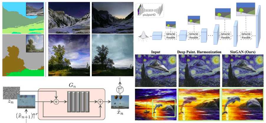
The generation of an image sample starts at the coarsest scale and sequentially passes through all generators up to the finest scale. The typical workflow of a single scale works like this: 5 conv. blocks followed by batch normalization and a ReLU activation process the upsampled image. Before the hallucinated image is fed in the network, noise is added. The spatial dimension is kept throughout the block, with padding of 1 and kernel 3 by 3. Therefore, a short additive skip-connection can be added, fusing the upsampled image to the output of the block. This concept significantly helps the model to converge faster, as we have already seen in a lot of approaches. All the above can be illustrated below:

Building block of the generator of one scale of SinGAN. Image is taken from the original work

Importantly, following other successful works (BigGAN, StyleGAN), noise is injected at every scale. The reason is that we don't want the generator to memorize the previous scale, since it’s training is stopped. In the same direction, the different GANs have small receptive fields and limited learning capacity. Intuitively, we don't want the patches to memorize the input, since we only train with a single image. Limited capacity refers to the small number of parameters.

As a reference, the effective receptive field at the starting level is roughly 50% of the image’s height. Thus, it can generate the general layout of the image (global structure). The pre-described block has a receptive field of 11x11, so usually input images start at the scale of 25 pixels.

Reconstruction loss

Interestingly, they chose to design the model in a way that when you choose zero as input noise and a fixed noise for the last layer (z_fixed) the network should be trained to reconstruct the original image.

L_{rec} = || G_{n}(noise=0,x_{upsampl}^{rec}) - x_{n}^{real} ||^2

L_{rec} = || G_{last}(noise = z_{fixed},x_{upsampl}^{rec}) - \textbf{I}^{real} ||^2

If we regard the real image as the zero point of the distribution the reconstruction loss is a measure of standard deviation. Therefore, the reconstructed image $x_rec$ determines the standard deviation of the noise for each scale.

Results and discussion

Inspecting the outputs of the model, we observe that the generated images are realistic, while they preserve the original image content. Since the model has a limited receptive field in each patch (smaller than the entire image), it is possible to generate new combinations of patches that did not exist in the input image. Below you can see how the model encounters the structure of externally injected models. We note that SinGAN preserves the structure of the pasted object, while it adjusts its appearance and texture.

SinGAN results on image harmonization. Image is taken from the original work

Based on the plenty results of this work, it is easy to infer that the SinGAN model can generate realistic random image samples. Surprisingly, even with new structures and object modulations. Still, it learns to preserve the image/patch distribution.

For the record, the authors have also explored SinGAN for other image manipulation tasks. Given a trained model, their idea was to utilize the fact that SinGAN learns the patch distribution of the training image. Hence, manipulation can be achieved by injecting an image into the generation pyramid. Intuitively, the model will attempt to match its patch distribution to that of the training image. Applications include image super-resolution, paint-to-image, harmonization, image editing, and even animation from a single image by “walking” the latent space!

The official video summarizes the aforementioned contributions of this work that we described in this tutorial.

Finally, the authors have released the official code, which can be found here.

Conclusion

We carefully inspected the top performing methods on image synthesis from a segmentation map, as well as learning from just a single image. For the hungry readers we always like to leave a thoughtful highly-recommended link. So, now that you learned a lot of things about what designing and training a GAN looks like, we recommend exploring the open questions on the field, perfectly described in this article by Odena et al. 2019. You can always find more papers that might be closer to your problem here. Lastly, you don't need to implement every architecture by yourself. There is an awesome GAN git repository in Keras and Pytorch that contains multiple implementations. Feel free to check them out.

This is the last article of the series for now. But note that the GANs in computer vision series will remain open to include new papers in the future, as well as existing ones we might have missed. We released a free e-book that summarizes our conclusions and concatenates all of our articles into a single resource. If you want to express your interest subscribe to our newsletter to receive it straight into your inbox. For a more hands-on course visit GANs coursera specialization.

Adaloglou Nikolas and Karagianakos Sergios

Cited as:

@article{adaloglou2020normalization,
  title   = "In-layer normalization techniques for training very deep neural networks",
  author  = "Adaloglou, Nikolas",
  journal = "https://theaisummer.com/",
  year    = "2020",
  url     = "https://theaisummer.com/normalization/"
}

For a hands-on video course we highly recommend coursera's brand-new GAN specialization.However, if you prefer a book with curated content so as to start building your own fancy GANs, start from the "GANs in Action" book!

References

Park, T., Liu, M. Y., Wang, T. C., & Zhu, J. Y. (2019). Semantic image synthesis with spatially-adaptive normalization. In Proceedings of the IEEE Conference on Computer Vision and Pattern Recognition (pp. 2337-2346).
Shaham, T. R., Dekel, T., & Michaeli, T. (2019). Singan: Learning a generative model from a single natural image. In Proceedings of the IEEE International Conference on Computer Vision (pp. 4570-4580).
Odena, "Open Questions about Generative Adversarial Networks", Distill, 2019.
He, K., Zhang, X., Ren, S., & Sun, J. (2016). Deep residual learning for image recognition. In Proceedings of the IEEE conference on computer vision and pattern recognition (pp. 770-778).
Kingma, D. P., & Welling, M. (2013). Auto-encoding variational bayes. arXiv preprint arXiv:1312.6114.
Chen, L. C., Papandreou, G., Kokkinos, I., Murphy, K., & Yuille, A. L. (2017). Deeplab: Semantic image segmentation with deep convolutional nets, atrous convolution, and fully connected crfs. IEEE transactions on pattern analysis and machine intelligence, 40(4), 834-848.

* Disclosure: Please note that some of the links above might be affiliate links, and at no additional cost to you, we will earn a commission if you decide to make a purchase after clicking through.

GANs in computer vision - semantic image synthesis and learning a generative model from a single image