For a comprehensive list of all the papers and articles of this series check our Git repo
For a hands-on course we highly recommend coursera's brand-new GAN specialization
Computer vision is indeed a promising application field for GANs. Until now, we focused on conditional and unconditional image generation. In the previous post, we provided a lot of aspects such as training with Wasserstein loss, understanding disentangled representations, modeling global and local structures with different strategies, progressive incremental training of GANs, etc. Nevertheless, deep learning in computer vision includes a variety of awesome tasks such as object generation, video generation, etc. We actually reached the point of megapixel resolution with progressive GANs for the first time. The question is: can we do better?
In this part, we will inspect 2K image and video synthesis, large-scale conditional image generation. Our extensive analysis attempts to bridge the gaps that you may have from previous works on the field. We will revise a bunch of computer vision concepts such as object detection, semantic segmentation, instance semantic segmentation. Basically, we would like to exploit all the available labels and highly accurate networks to maximize visual quality. That means even the ones that can be generated from state-of-the-art deep learning models. Since 2018 GANs gained increased attention in the community due to their avast cool applications, especially in computer vision. Nevertheless, one easily grasps that since the introduction of progressive GANs at the end of 2017, NVidia started to own GANs in computer vision! We will analyze the following three foundational works:
pix2pixHD (High-Resolution Image Synthesis and Semantic Manipulation with Conditional GANs 2017)
As you can imagine this work extends the pix2pix model that we discussed in part 2. In essence, the pix2pix method adopts a symmetric u-net architecture for the generator and a patch-based discriminator. More importantly, the input to the discriminator is both the input image and the generated one (i.e. concatenation of image with semantic label). Nevertheless, the image resolution reaches up to 256 × 256, which is still low. It is widely known in computer vision that a multi-resolution pipeline is a well-established practice, with two-scale approaches to dominate because it is often enough to model 2 scales.
But how did they manage to improve pix2pix in a multi-scale fashion?
Decomposing the generator
The generator G is decomposed in G1 and G2. G1 acts as the global generator network and G2 acts as the local enhancer network. G1 operates in a lower dimension, specifically half of the dimension of G2 in each spatial dim. Out of the box, it can be seen close to the idea of progressive GANs, but instead of symmetrically adding higher operating layers for both G and D, they enhance this idea just in the generator architecture.
G1 and G2 are trained separately and then G2 is trained together with G1, similar to a two-step progressive GAN with much bigger building blocks. As you will start to understand, more and more attention will be given to the careful design of the generator. A visual illustration can be seen below:
 The generator of pix2pixHD, borrowed from the original publication.
Global Generator G1: In this direction, they adopted and built upon an already successful architecture in 512x512 resolutions. G1 alone is composed of 3 components:
A convolutional front-end architecture G1_front, that decreases the spatial dimensions.
A large set of skip residual blocks G1_res, that the heavy processing is performed.
A transposed convolutional back-end G_back that restores spatial dimensions.
In this sequential manner, a segmentation map of resolution 1024×512 is passed through G1 to output an image of resolution 1024 × 512.
Local enhancer network G2: G2 follows the same 3-component hierarchy, with the first difference being that the resolution of the input is 2048 × 1024. Secondly, the input to the residual block G2_res is the residual connection (element-wise sum) of two feature maps:
the output feature map of G2_front (left black rectangle in the figure), and
the last feature map of G1_back
In this way, the integration of global image information from G1 to G2 is achieved. Now, G2 can focus on learning the high-level frequencies that correspond to the local details.
Let’s move on to see the design modifications and their reasoning for the choices of D.
Multi-scale discriminators
The motivation lies in the fact that the discriminator needs to have a large receptive field. To achieve this with convolutional layers, you can either add more layers, increase kernel size, or use dilated convolutions. However, these choices require high computational space complexity, which is intractable for such high-resolution image generation.
But let’s start our analysis with an observation. What would happen if we don't use multiple discriminators? The authors highlight that without the usage of multi-scale discriminators, many repeated patterns are often observed. To this end, the authors use 3 discriminators (D1, D2, D3), that have an identical network structure. Still, they operate at different image scales.
In more details, both the real and synthesized high-resolution images are downsampled by a factor of 2 and 4. Therefore, we now have 3 scales of image pairs, namely 2048x1024, 1024x512, 512x256. This is usually called an image pyramid in computer vision terms.
The discriminator D1 that operates at the coarsest scale(highest resolution) has the largest receptive field. Therefore, it is obvious that it perceives a more global view of the image. This can aid the guidance of the generator (especially the global gen. G1) to ensure global consistency in the images. In the opposite direction, the discriminator D3 at the finest scale encourages the generator (especially the local enhancer G2) to model finer local details.
So, we have a multi-scale G and D. Let’s now explore an exciting way to match their scales in a feature-loss manner.
Multi-scale feature matching loss
Feature matching loss enables G to match the expected value of the features on an intermediate layer of the discriminator. This objective requires the generator to generate data that matches the statistics of the real data, here in multiple scales! By training the multi-scale discriminator in this fashion, we ask D1, D2, D3 to find the most discriminative features of real data versus the generated ones. Consequently, multi-scale feature loss stabilizes the training as G has to produce multi-scale natural statistics. Let’s see the math:
In the above equation, T is the layers of each discriminator and N is the number of elements of the feature map of each layer. Indexing D with k shows that this loss can be applied in all the discriminators. s is the input image(i.e. segmentation) and x is the real target data. Notice again that D has access to both input and hallucinated images. For 3 D’s we have three feature matching losses, operating at different scales.
Using semantic instance segmentation
First, let’s start by ensuring that we understand the types of segmentation and detection:
Object Detection: We detect an object, usually with a bounding box(2-pixel locations) in an image.
Semantic Segmentation: We classify each pixel in a class(category), called semantic labels (i.e. cars, trees)
Instance Segmentation: We extend semantic segmentation by further identifying the class instance it belongs to (i.e. Car 1, Car 2, Tree 1 Tree 2, etc...) So, an instance-level segmentation map contains a unique class ID for each individual class (object).
 Taken from Silberman et. al 2014 (ECCV). Paper can be found here link.
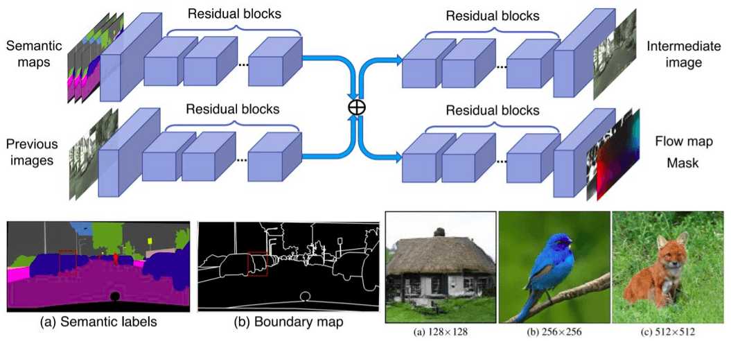
Based on the above, it is obvious that segmentation maps do not differentiate objects of the same category. The authors believe that the most crucial information which lies in the instance map is the object boundary. Let's see how you can create such a boundary map.
In their implementation, a binary instance boundary map can be formed as simply as this: a pixel has a value of 1 if its unique class ID is different from any of its 4-neighbors, and 0 otherwise.
 Boundary map from instance-level segmentation maps, taken from pix2pixHD
Let’s focus on the red rectangle in the illustrated images. When we have a series of cars with the same semantic label, semantic segmentation is not enough. By using instance labels and looking in the neighbors, one can derive a binary boundary map.
The instance boundary map is then concatenated with the one-hot vector representation of the semantic label map, and fed into the generator network as one more input channel. This method might seem simple and intuitive, but in practice, it works extremely well, as depicted below:
 Exploiting hand-crafted instance-based boundary maps, taken from here
Learning an Instance-level Feature Embedding
Moving one step further it is possible to learn and embed such maps in the input of the generator to increase diversity that guarantees image and instance-level consistency. Instead of feeding hand-crafted maps such as the binary boundary map, we can train a network to produce diverse feature embeddings. Let’s summarize the process of generating the low-dimensional features:
We train an encoder E(x) to find a low-dimensional feature vector. The latter should correspond to the ground truth for each instance in the image. Note that x is the real image.
So, we add an instance-wise average pooling layer to the output of the encoder to compute the average feature for the object instance. This ensures that the features are consistent within each instance.
The resulting average feature is broadcasted to all the pixel locations of the specific instance. For example, all pixels that refer to car 1 will share a common average feature, which will be different from car 2.
We replace G(s) with G(s | E(x) ) and train the encoder jointly with the generators and discriminators.
After training, we run it on all instances of the training images and save the obtained features (offline!).
For each semantic category (NOT instance) we perform a K-means clustering on all features. So, we have a set of K clusters that correspond to different representations of each category. This can be regarded as: each cluster encodes the features for a specific style of the same instance.
For inference, we can just randomly pick one of the cluster centers and use it as the encoded continuous features.
All the above can be illustrated in practice in this image (road style and main car style are changed based on this methodology):
 Results of pix2pixHD GAN by introducing instance-level feature embeddings
Finally, it is highlighted that the pix2pixHD learns to embed the style of different objects, which can be proven beneficial to other application domains, that pre-trained models are not available. Further results and official code are provided on the official site.
Video-to-Video Synthesis (2018)
We already saw a bunch of beautiful image generation. But what about video generation? In this exciting work, the authors tackle the novel task of video-to-video generation.
Basically, we are conditioning on the previous video sequence as well as their corresponding segmentation maps. But let’s see why this task introduces some really difficult challenges. One may argue that you can just use the best high-resolution conditional image prediction, which is pix2pixHD.
Even though this broad category of models achieves impeccable photo-realistic results, the resulting stacked video lacks temporal coherence. The roads, buildings, and trees may appear inconsistent across frames. The main reason that we observe these visual artifacts is because there is no constraint that guarantees temporal consistency (across frames).
An awesome illustration of video incoherence is illustrated in the official video.
Formulating the problem in terms of machine learning
In video synthesis, we aim to learn a mapping that can convert an input video to an output video. Mathematically, given a pair of segmentations maps s and RGB videos x we want to generate a sequence y conditioned on s so that: p(x|s) = p(y|s).
By expressing the problem as conditional sequence distribution matching, it is possible to learn the desired temporal coherence. To this end, the authors model the problem by factorizing p(y|s) as a product of the probabilities of the last two timesteps.
We index the new timestep of the video by index 3, and the two previous timesteps as 1 and 2 throughout this tutorial. This notation is adopted to simplify the explanation. However, this approach can be generalized to take into account more frames.
More specifically frames are produced sequentially given:
current segmentation mask (s3)
the past two segmentation masks (s1,s2)
the past two generated frames (x1,x2)
This conditional assumption is called the Markovian assumption. It is basically the conditional independence assumption for sequences. For this reason, we use a deep network to learn this mapping called F. Hence, we can obtain the final video by recursively applying F. Is this alone enough to produce a state of the art 2K resolution video generation? Of course not! Let’s see some more magical engineering.
Generator: Exploiting optical flow
It is known that consecutive frames contain a significant amount of redundant information. How can we optimize this? If optical flow information (W) was available, it would be possible to estimate the next frame by a simple process called frame warping. If you are not familiar with optical flow concepts, you can quickly check here.
Now, we have a new problem. Optical flow warping is an estimation that fails in occluded areas but works well on the other parts of the image. Ideally, we would need an additional mask (M) to inform us about the occluded and non-occluded pixels so that we can use optical flow.
And even if all the above were possible, we would still need an image generator (H) to generate image h, focusing on the occlusion pixels.
Unfortunately, we don’t have this information. Fortunately, since we use deep learning models, it is possible to use pre-trained state-of-the-art models for W and M, namely Flownet2 and Mask-RCNN. These models produce w(x) - warped image of x, given optical flow network W- and m (soft mask), respectively. It is worth mentioning that the produced masks are soft masks (continuous in a specified range). Therefore, the network slowly adds details by blending the warped pixels and the generated pixels.
Finally, we can express the problem like this:
where m’ is the inverse mask, w the warped image of x2, estimated from W, and h the hallucinated image from the generator H.
 An illustration of the generator components, taken from the original paper
All the above models M, W, and H use short residual skip connections. The generator is similar to pix2pixHD in order to cope with high-resolution images. An excellent official repository is available from NVidia here.
Discriminator: facing the spatio-temporal nature
Since the problem is spatio-temporal, one way to design it is by dividing it into two sub-problems. It is known that you can use more than one discriminator, whereas each one focuses on different sub-problems. In our case, the problem is decomposed as discriminating images and videos.
We will refer to the conditional image discriminator as DI and the conditional video discriminator as DV. Both follow the principle of PatchGAN from pix2pix, which means that the adversarial learning is calculated for some part of the input. This idea makes training faster and models detailed and localized high-level frequencies (structures).
On one hand,DI is fed with a single pair of segmentation mask and an image (video slice) and tries to distinguish the generated images. The pair is uniformly sampled from the video sequence. On the other hand, DV is conditioned on the flow to achieve temporal coherence. That’s why it is fed with pairs of a sequence of images and a sequence of optical flows. The patches are generated by choosing k consecutive frames from the sequence. The sampling technique is crucial here, as it makes computations more tractable by lowering the time and space complexity.
Moreover, given a ground truth of optical flows, one can calculate an optical flow estimation loss to regularize training. Finally, the authors use the discriminator feature matching loss as well as the VGG feature matching loss, similar to pix2pixHD. These widely accepted techniques regularize further the training process and improve convergence speed and training stability. All the above can be combined to achieve the total optimization criterion to tackle video synthesis. The official video that follows might convince you more:
Further distilling performance from semantic segmentation masks
Semantic segmentation treats multiple objects of the same class as a single entity. So, it is possible to divide an image into foreground and background areas based on the semantic labels. For instance, buildings belong to the background, while cars belong to the foreground. The motivation behind this is that the background motion can be modeled as a global transformation. In other words, the optical flow can be estimated more accurately than the foreground. On the contrary, a foreground object often has a large motion, which makes optical flow estimation ineffective. Therefore, the network has to synthesize the foreground content from scratch. This additional prior knowledge significantly improves the visual quality by a large margin, as you can see below (bottom left is the vid-to-vid model).
 Results from vid-to-vid GAN, taken from the original work
What about instance semantic segmentation?
This process is heavily based in pix2pixHD. Instance segmentation treats multiple objects of the same class as distinct individual objects. How could you possibly add stochasticity to produce meaningful diversity in this huge model?
One way to do so is by producing a meaningful latent space. This is possible through feature embedding. Practically, to map each instance (car, building, street) to a feature space.
This is done via a convolutional layer followed by a custom instance-wise average pooling layer in the input image, to produce a different feature vector for each instance. But isn't this a latent space vector that can be used to introduce stochasticity? Yes, it is! Therefore to introduce stochasticity in the model (multimodal synthesis), the authors adopt the aforementioned feature embedding scheme of the instance-level semantic segmentation masks.
This latent feature embedding vector is fed along with the segmentation mask to F. In this way, one can fit a different distribution for each instance (i.e. Gaussian) so that he can easily sample from the desired instance at test time to produce instance-wise meaningful diversity! The official code has been released here.
 The road instance is changed in the video. Taken from the original work.
BigGAN (Large Scale GAN Training for High Fidelity Natural Image Synthesis 2018)
What would you do to improve a generative network, if you had all the computing power and time in the world? You would probably want to use them as effectively as possible with the best techniques that scale up well. We referred to megapixel resolution for unconditional generation, but what happens when we want to have class-conditional high-resolution image generation?
This work tackles conditional image generation on really large scales. It is well-known that instability and mode collapse are harder problems to solve in the class-conditional setup. Even though the official TensorFlow implementation (with pre-trained weights) is available, I would not bet that you can deploy these models on a single GPU. By the way, another awesome accompanying PyTorch repo with more realistic requirements is provided here.
Summarizing large-scale modifications
Let’s briefly summarize the different techniques and tricks of this work.
Incrementally scaling up to a maximum of 4 times the parameters compared to previous models.
Scaling up batch size up to 8 times (2048!) with a distributed training setup.
Use an existing well-performing GAN, namely SA-GAN, and increase its feature maps and depth.
Employ the best normalization technique for GANs, namely spectral normalization
Use the effective hinge loss, described in detail here
They provided class information with an already established technique, called conditional-batch norm with shared embedding, described here and here
They used orthogonal initialization for the parameters.
They lower the learning rates and make two D steps per G step.
They finally add a skip residual block structure to increase network depth effectively, because of the vanishing gradient problems.
Last but not least, they introduce the so-called truncation trick!
Increase batch size
Increasing the batch size provides better gradients for both networks. Applying only this particular modification of increasing the batch size by a factor of 8 improves the performance score by 46%. One notable side effect is that the proposed model reaches the final performance in fewer iterations, but with additional instabilities.
Increase the width
Moreover, by increasing the number of channels (feature maps) by 50% the total number of trainable parameters is doubled. Batch-norm with conditional shared embedding, reduces time and space complexity, as well as it improves the training speed. Consequently, the width increase leads to an additional 21% improvement.
Increase depth
To increase the network’s depth, they designed direct skip connections from the noise vector z to multiple generator layers, called skip-z. The intuition behind this design is to allow G to use the latent space z to directly influence features at different resolutions and levels of hierarchy. In the bigger models, they simply concatenate the z with the conditional class vector. Amazingly, skip-z connections provide 4%, while speed up training by 18%!
Truncation Trick
Given the initially sampled vector z that is sampled from a normal distribution, one can compute the vector norm (magnitude). The idea is to resample the vector if the calculated magnitude is not above a fixed hardcoded threshold (i.e. 1). This is performed only in the already trained model. As a result, they experimentally observed that this minor change leads to a significant improvement in individual sample quality at the cost of reduced diversity. However, this trick can be problematic for some models. To face this issue,the authors try to constrain G to be smooth, so that all the range of z will map to good output samples. That’s why they employ orthogonal regularization.
Results
All the aforementioned modifications lead to the state-of-the-art class-conditioned image generation, illustrated below:

A critical finding is that stability comes from the balanced interaction between G and D through the adversarial training process. Moreover, Big-GAN interpolates with success between same-class samples, suggesting that it does not simply memorize training data. Another important observation that is derived from this study is the class leakage, where in images from one class contain properties of another. This may be justified due to the huge batch sizes. Finally, it is also worth noticing that many classes that exist in large portions and are distinguished by their texture (i.e. dogs) are easier to generate. On the other hand, limited portion-classes that have more large-scale structures (crowds) are harder to generate.
Conclusion
In this tutorial, we inspected some of the top-performing GANs in computer vision for 2018. We provided a wide perspective of the best techniques in the field, rising naturally from tackling real-world large-scale problems. We started with a 2K image generation and multiple generators and discriminator. Then, we moved to video synthesis conditioned on past frames with guaranteed temporal consistency. Finally, we revisited class-conditioned image generation in ImageNet, taking into account all the engineering tricks known in the field.
For our math-keen GAN readers, we encourage you to take a good look at Spectral normalization in GANs, which we did not cover in this tutorial. Another relative computer vision application of GANs is StarGAN, which is pretty interesting to investigate also. There is no one size fits all. Find the best method that tackles your problem. We really hope that this tutorial series provides you with a clear overview of the field.
Still, there is an infinite set of directions to explore, as we will see in the next part.
For a hands-on video course we highly recommend coursera's brand-new GAN specialization.However, if you prefer a book with curated content so as to start building your own fancy GANs, start from the "GANs in Action" book! Use the discount code aisummer35 to get an exclusive 35% discount from your favorite AI blog.
Cited as:
@article{adaloglou2020gans,title = "GANs in computer vision",author = "Adaloglou, Nikolas and Karagiannakos, Sergios ",journal = "https://theaisummer.com/",year = "2020",url = "https://theaisummer.com/gan-computer-video-synthesis/"}
References
- Wang, T. C., Liu, M. Y., Zhu, J. Y., Tao, A., Kautz, J., & Catanzaro, B. pix2pixHD: High-Resolution Image Synthesis and Semantic Manipulation with Conditional GANs.
- Wang, T. C., Liu, M. Y., Zhu, J. Y., Liu, G., Tao, A., Kautz, J., & Catanzaro, B. (2018). Video-to-video synthesis. arXiv preprint arXiv:1808.06601.
- Brock, A., Donahue, J., & Simonyan, K. (2018). Large scale gan training for high fidelity natural image synthesis. arXiv preprint arXiv:1809.11096.
- Johnson, J., Alahi, A., & Fei-Fei, L. (2016, October). Perceptual losses for real-time style transfer and super-resolution. In European conference on computer vision (pp. 694-711). Springer, Cham.
- Silberman, N., Sontag, D., & Fergus, R. (2014, September). Instance segmentation of indoor scenes using a coverage loss. In European Conference on Computer Vision (pp. 616-631). Springer, Cham.
- Ilg, E., Mayer, N., Saikia, T., Keuper, M., Dosovitskiy, A., & Brox, T. (2017). Flownet 2.0: Evolution of optical flow estimation with deep networks. In Proceedings of the IEEE conference on computer vision and pattern recognition (pp. 2462-2470).
- He, K., Gkioxari, G., Dollár, P., & Girshick, R. (2017). Mask r-cnn. In Proceedings of the IEEE international conference on computer vision (pp. 2961-2969).

* Disclosure: Please note that some of the links above might be affiliate links, and at no additional cost to you, we will earn a commission if you decide to make a purchase after clicking through.