For a comprehensive list of all the papers and articles of this series check our Git repo
For a hands-on course we highly recommend coursera's brand-new GAN specialization
The previous post was more or less introductory in GANs, generative learning, and computer vision. We reached the point of generating distinguishable image features in 128x128 images. But if you really want to understand the progress of GANs in computer vision you definitely have to dive into image to image translation. Although this are the first successful models their principles to design a GAN are still taken into consideration.
So, in this part, we will continue our GAN journey in computer vision inspecting more complex designs that lead to better visual results. We will revisit mode collapse, 3D object generation, single RGB image to 3D object generation, and improved quality image to image mappings. Let's just jump in the contents!
AC-GAN (Conditional Image Synthesis with Auxiliary Classifier GANs 2016)
This amazing paper presents comprehensively the first attempt to produce detailed high-resolution image samples (for that time 128x128) with high variability among the class (intra-class variability). As we have already seen, the class is the conditional label. In this work, a GAN was trained that simultaneously tries to generate 10 different classes!
It is known that when you try to force a model to perform additional tasks (multi-task learning) the performance on the original task can be significantly increased. But, how can you do it? Using reconstruction loss!
Auxiliary or reconstruction loss
Combining the ideas of InfoGAN (information regularization) and conditional GAN (use image labels), the AC-GAN is an extension of GAN that uses side information (provides image class). Instead of just providing G and D with the conditional information, they let D to learn to reconstruct this side information (the so-called reconstruction loss).
Specifically, they modified D to contain an auxiliary (extra) decoder network that can utilize pre-trained weights from a standard classification setup. The auxiliary decoder network outputs the class label for the training data. That way, synthesizing image quality is greatly improved. The AC-GAN model learns a representation for noise (z) that is independent of the class label, therefore not necessary at the inference time of the generator.
Furthermore, the particular reconstruction objective, even though it is quite simple, appears to stabilize training. Training an ensemble (multiple models) of 100 AC-GANs, wherein each model is trained on 10 different classes, the ensemble AC-GANs generate 1000 realistic image classes (from Imagenet 1K dataset)
A common evaluation technique that is really important to understand is the inception score that we saw on the previous part 1. For self-completeness let’s briefly recap: you use a pre-trained model to measure the correct classification of class-conditionally generated images. Inception score measures discriminability. Surprisingly, the authors found that synthesizing higher-resolution images leads to increased discriminability (up to 128x128 spatial resolution). But what about sample diversity?
Structural similarity
In computer vision and image processing we commonly use this metric to evaluate noise and distortion. SSIM is a perception-based model that considers structural information through image statistics, namely mean and standard deviation. SSIM incorporates important visually perceived phenomena.
In an attempt to evaluate the diversity of generated images, multi-scale structural similarity (MS-SSIM) was adopted. Even though this metric was initially introduced for image compression, it is experimentally shown that it is also a sufficient metric to evaluate generated image quality.
Less literally, higher diversity results in lower mean MS-SSIM scores. Ideally, we would like same-class generated images to have low similarity--> high diversity! To increase intuitive understanding, we will just refer to MS-SSIM as similarity.
It is important to understand that structural information is strongly related to image statistics. We are aware that pixels have strong inter-dependencies, especially when they are spatially close (that’s why we designed image convolutions and work extremely well anyways 😊).
 Taken from AC-GAN
Synthesized data don’t have the diversity of training samples, as shown, because they have a higher score. Still, they definitely move in the right direction. To conclude, even though this metric is relatively easy to compute, it is a significant measure of perceptual diversity of the generated outputs, so as to be sure that the model did not memorize the training data. There are, however, a lot of other ways to validate that, as we will see.
Discussion points
- It is not enough to introduce the metrics but also to understand the relationship between the data through it. Below, we can see a super intuitive plot of similarity (MS-SSIM) and accuracy. The red line is the average diversity of the real data. The majority of high similarity classes do not yield improved accuracy, while the majority of low similarity (high intra-class diversity) yields an accuracy between 1% and 20%. This fraction may sound low but keep in mind that even the real data have a ~77% inception score in ImageNet. This finding contradicts the general impression that GANs achieve high sample quality at the expense of variability of that period. Still, for images up to 128x128! This shows the big learning capability of AC-GAN.

- Condition and noise (or better walking the latent space): When a generative model overfits the real distribution, one is able to observe sharp and discrete transitions in the sampled images. Furthermore, there are usually regions in the latent space that do not correspond to meaningful content. In the image that follows, if you look from left to right you can see samples with the same sample noise but with a different class condition of 8 bird categories. It is crucial to understand that non-related structure that relates to image structure is maintained. On the contrary, looking in the contents of the column one can observe same-class samples with different noise vector. Class-related characteristics are consistent throughout the different noise samples.

It is unclear what is the best way to divide a dataset for a generative model to learn only a subset of classes. However, restricting the number of classes from 1000 to 10 improves quality, even though a single class generative model can be really unstable. We show that in the previous tutorial by training a DCGAN in one CIFAR10 class, wherein we observed mode collapse.
Finally, since the generator doesn’t need class-information to provide samples, the AC-GAN can be used pretty straightforward in a semi-supervised setup.
3D-GAN (Learning a Probabilistic Latent Space of Object Shapes via 3D Generative-Adversarial Modeling 2017)
Is it possible to leverage the existing advances on volumetric (3D) convolutional networks along with generative adversarial networks? This wonderful work says that it is not just possible, but it is also really effective.
Understanding the problem of 3D object generation
3D object generation is a more challenging problem than image generation. Compared to the space of 2D images, it is more difficult to model the space of 3D shapes. To quantify this, think that 64x64 equals 4096 pixels, while 64x64x64 equals 262144 voxels. This is what we mean by higher dimensionality in practical terms
To limit the increasingly high number of parameters, authors choose to use only convolutional blocks. Surprisingly, there are no pooling layers. The proposed model is basically an extension of DCGAN with volumetric convolutions, as depicted in the figure below:
 3D-GAN generator taken from here.
As depicted in the picture, each convolutional layer of kernel size 4x4x4 and stride of 2. This conv3d layer doubles the 3D dimensions while reducing the number of features by a factor of 2. As in DCGAN, the discriminator uses a symmetrical architecture with Leaky Relu activations instead of ReLU. Our Pytorch re-implementation of 3D-GAN is available here
Training strategy
The basic novel part of this work comes in the training strategy. Since generating objects in a 3D voxel space is more difficult than classifying them, there is a training imbalance between G and D. As you can imagine, in such cases, it is possible that D learns faster than G. To alleviate this problem, three small tricks are utilized. First, the usage of a lower learning rate in D than G. Second, a relatively big batch size of 100, which is huge for a 3D network! Finally, the discriminator only gets updated only if its accuracy in the last batch is not higher than 80%. These tricks may be simple and task-defined but produce stable high-quality 3D objects.
Moving one step further
All the previously-described approaches in this article-series use random noise (z) with or without condition. However, let’s think what could happen if we could design the random noise z to be something more meaningful. For 3D object generation, it would be super cool to infer the latent vector z from an observation. Let’s think this through!
What if we project a 2D image in a trainable manner to produce z? That extra mapping would result in a transformation of a 2D image to a voxelized 3D object. Following the successful idea of VAE-GANs, they add an additional 2D image encoder, which outputs the desired latent representation vector z. To summarize, the total loss includes the adversarial loss (binary cross-entropy) and two more loss terms related to the variational autoencoder. The VAE losses refer to a) the KL divergence between the variational distribution of the latent representation and the prior distribution, and b) the reconstruction loss of mean square error between the generated 3D object from the image and the real one. Nevertheless, in order to train the 3D-VAE-GAN, pairs of 2D images and 3D models are required!
Tasks, results, and discussion
Based on all the above, the proposed model can be utilized in 3 tasks, that correspond to the 3 different components:
3D Object Generation using G
3D Object Classification using D
Single Image 3D Reconstruction!
We will only present the results of the latter because it is the most attractive task and visually appealing. For more demonstrations, there is also an interesting video. For our hardcore beloved software engineers, the official repo is also available here, although I would not recommend it.
 Based on the original work of 3D-VAE-GANs
It is really beautiful to understand the results of GANs, which this post is really focused on. We already discussed “walking” in the latent space and observing meaningful patterns of solutions between generated samples. By the way, the official terminology is interpolating the latent space between object-vectors.
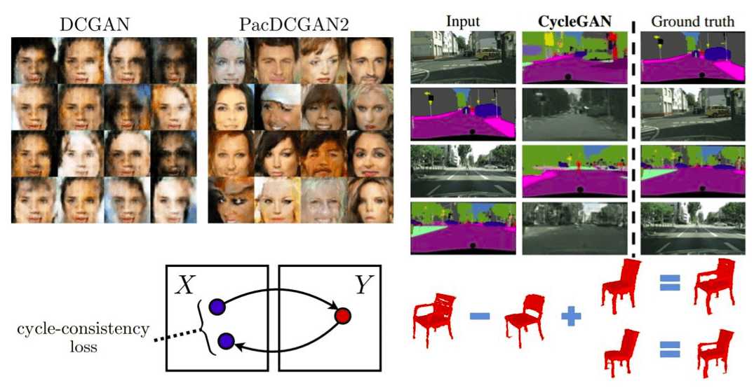
An even more great illustration that I personally adore in the field of GANs is the latent space arithmetic. Essentially, this consists of the idea that simple object-vector arithmetic operations can have a meaningful impact on the 3D voxel space. It is proven and shown that you can add or subtract different z vectors that correspond to appealing 3D objects so as to generate new ones that abstractly share the arithmetic operations of the low-dimensional space in the high dimensional space. A similar approach was illustrated in the disentangled representations of InfoGAN. Here, it is further generalized to arithmetic operations in latent space that lead to highly semantic content in the 3D space.
 Based on the original work of 3D-VAE-GANs-2
PacGAN (The power of two samples in generative adversarial networks 2016)
This work tackles the problem of mode collapse. Several other approaches rely on modified architectures, loss functions, and optimization to tackle it. However, it is not well understood how the proposed changes relate to mode collapse. This work introduces some foundational mathematics, based on binary hypothesis testing that efficiently explains and resolves mode collapse. I would say that this work takes the idea of minibatch discrimination of the paper Improved Techniques for Training GANs (2016) that we will analyze20 steps further.
Core idea
Instead of using a discriminator D(x) to map a single input to a single label, authors use a modified discriminator D(x1,x2, . . . ,xn) that maps n samples together, independent of their source domain(real or fake but not a mix of them). These samples are drawn independently from the same distribution, real or generated. It is important to understand that this approach is not related to batch size training.
The drawn samples are rather concatenated and are assigned a single label, which is the so-called packing. The concatenation is performed in the channel dimension for convolutional-based discriminators. To cope with that, the only modification is performed at the input of D by increasing the size of the convolutional kernels.
Intuition and some results
More intuitively, packing aids the discriminator by feeding him with a set instead of single images. It is believed that in this way D is able to detect mode collapse because the lack of diversity is more obvious. Mathematically speaking, this method allows the discriminator to do binary hypothesis testing based on the product of the distributions.
 The image is taken from the original paper.
As depicted, packing significantly improves the diversity of samples. As shown, the images generated from DCGAN and PacDCGAN2 are more diverse and sharper, with roughly the same number of parameters. Finally, officially published code can be found here.
Pix2Pix GAN (Image-to-Image Translation with Conditional Adversarial Networks 2016)
In this manuscript, authors move from noise-to-image (with or without condition) to image-to-image, which is now addressed as paired image translation task. Simply, the condition is an image and the output is another image. Noise sampling that was previously required to provide stochasticity and variability is removed, so the model learns almost deterministic mappings. It almost derives from the fact that they kept the training behavior of dropout and batch normalization layers in test time. However, this method does not provide great variability. Moreover, the discriminator has now access to an image pair(condition input image + real or generated).
Unet shape generator
It is important to perceive why they used this generator. Actually, the design of the generator is based on the assumption that both input-output images are renderings of the same underlying structure ( i.e edges). This means that there is low-level information that is shared, hence symmetrical skip connections are implemented between the encoder and the decoder of the generator, in an unet style architecture.
Furthermore, they provided an extra L1 loss (sum of absolute differences) loss between the generated image and the ground truth. In this way, they argue that the image quality will be higher since L1 loss leads to less blurring than L2 loss. Even though we discussed that this error without the adversarial terms is not effective, in this work they are used together. Let’s see why they bring back this idea!!!
PatchGAN discriminator
Intuitively, L1 and L2 losses are able to accurately capture the low frequencies (i.e. edges). Therefore, in this way the GAN discriminator is restricted to mostly model high-frequency details and structure. As stated, modeling high-frequencies is related to local information that can be found in small image sub-regions that we call patches. To that end, they choose a convolutional discriminator that receives multiple generated-image patches and averages the predictions to provide the scalar output of D. That’s why it is called PatchGAN! Now, let’s see some results!
 Image is taken from the original paper. The discussed details can be visually observed in the above image. Adding the L1 loss increases image quality, capturing low-level frequencies.
Cycle-GAN (Unpaired Image-to-Image Translation using Cycle-Consistent Adversarial Networks 2017)
All the previously described architectures for conditional image generation require training pairs. This work introduces the first breakthrough of unpaired conditional image generation. As opposed to previous approaches, this model learns a mapping from a set (collection) of images to another set of images. Of course, this can be addressed by the assumption that the set contains repeated patterns and characteristics that can be learned. The question is if it is possible to learn such a cool mapping (translation of images to images) in the absence of paired examples. Even though there exists an assumption that there must be some kind of correlation between the two collections, it is still a challenging task! From now on, we call the collections of input and output sets of images, domain X and Y, respectively. Formulating the problem in this manner, our new task is domain mapping!
The bad news of domain mapping
In general, this approach has an inherent problem. The mapping (G) that we want to learn does not guarantee consistency at an individual level. Specifically, we don’t have any constraint that an individual input image of domain X and a generated image of domain Y are paired meaningfully. The previously-described observation is derived from the fact that there are infinitely mappings G that will provide the same output, unlike individual mapping of previous methods. Intuitively, we are looking in a much more abstract and complex world (latent space). The first experiments of this world introduced by this great work, validate the complexity by encountering instability and mode collapse, as expected!
The good news of domain mapping: introducing cycle consistency
Generalizing to domain mapping introduces new challenges. To this end, authors exploit the property that the learned translation should be “cycle consistent”. Let’s dive into this idea a little bit more.
Instead of learning a single mapping G: X --> Y, we could also learn the inverse domain mapping, called F, such that F: Y --> X. How does learning this mapping alone can help us? Does it constrain G? The answer is NO! At least not alone.
However, there is a better side. We can play around with these to map and make domain “cycles”. Let's start by taking the conditional image x (in X domain) and translate it with G back to the desired Y domain. The big question comes now: What if we take this generated image y that is supposed to live in domain Y and apply again the mapping F. What will the output be now? Think about it along with this helping figure.
 Making cycles in domain X, borrowed from the original work for intuitive understanding.
So, if we were living in an ideal world, I can assure you that we would get back the input conditional image. This is the core idea of this wonderful paper! Mathematically, F(G(x)) = x and G(F(y)) = y. Surprisingly, it is the same idea by 1-by-1 functions that you learn in basic calculus!
Since we don’t have the ideal mapping, because we are not in an ideal world, let us minimize this distance between these quantities. Namely, let’s minimize the L1 distance of F(G(x)) and x as well as G(F(y)) = y. Of course, there are a lot of ways to minimize the distance between an individual set of the domain. The most straightforward measure that yielded the best results was the 1st norm: the sum of absolute differences defined as:
The expected value is used because of the stochasticity of the GANs, which usually comes from random noise (but not in this work!). Therefore, let us teach two GANs (4 deep networks) to learn these mappings, combining their adversarial losses with the illustrated cycle-consistent constraint. Adding together 2 adversarial losses with the proposed cycle loss, with another scalar hyperparameter, one can have the full training objective. There are application-specific cases that we need to preserve color composition between domains, so the identity loss term is added to the equation. Implementations of Cycle-GAN and Pix2Pix can be found in this well-maintained GitHub repo here.
Results and discussion
As you can see, the results are of course impressive. In the first figure, it is illustrated that both mappings are learned. There is some blurriness in the images, but you have to think about the complexity of the problem.
 Image is taken from the original paper
Even compared with a paired approach, which is clearly an unfair comparison, such as pix2pix, we can see that the results are worse but still competitive.
 Image is taken from the original paper
In my humble opinion, it is exciting to see top works like this clearly exposing the limitation of their own methods. This is a rare asset in top-quality deep learning research that I admire! In general, the results bring a lot of hope in the field. However, for tasks that require large geometric changes, this approach has proven to have limited success. One reason might be that this approach captures more global characteristics of the domain. This can be interpreted as learning the global characteristics is the first step of the domain mapping. Moreover, there is no explicit paired guidance to enable local information extraction. Simply, the model is not constrained in this aspect.
Other visually-observed failure cases are caused by the distribution particularities that may exist in the training datasets. This expected observation is related to the described assumption of the repeated patterns and characteristics between domains. Still, the paired image-to-image translation remains an upper boundary for the unpaired approaches. Finally, there is an enormous number of available unpaired images that one can use with this method.
Cycle GAN training scheme pseudo Python code for intuitive understanding
We decided that since we have 2 GANs there might be confusion in how the training of such a model might work. That’s why we brought you an actual python code that helps in understanding the training process. It is important to clarify that the code was borrowed from the original repo, although severely altered to maximize the understanding of the concepts. There are comments so that you can read around the code. Some functionality is not filled to keep the size limited while focusing on the new important aspects. So, you will see that some parts are abstractly defined.
import torchimport itertoolsclass CycleGAN():def init(lr_g, lr_d, beta1, fake_pool_X, fake_pool_Y, criterionGAN, criterionCycle):"""Define any G image-to-image model and any D image-to-scalar in [0,1]"""self.netG_X = generator()self.netG_Y = generator()self.netD_X = discriminator()self.netD_Y = discriminator()# Unify generator optimizersself.optimizer_G = torch.optim.Adam(itertools.chain(self.netG_X.parameters(),self.netG_Y.parameters()), lr=lr_g, betas=(beta1, 0.999))# Unify discriminator optimizersself.optimizer_D = torch.optim.Adam(itertools.chain(self.netD_A.parameters(),self.netD_B.parameters()), lr=lr_d, betas=(beta1, 0.999))self.hyperparameters = (lambda_X,lambda_Y)# Abstractly defined Image-pooling and criteria# for code-compactness and understandingself.fake_pool_X = fake_pool_Xself.fake_pool_Y = fake_pool_Yself.criterionGAN = criterionGANself.criterionCycle = criterionCycledef training_cyclye_gan_scheme(real_X_data, real_Y_data):"""real_X_data is a bunch(mini-set) of images from domain X.real_Y_data is a bunch(mini-set) of images from domain Yshape is [batch, (mini-set), channels=3, height, width]"""# we make input data available as class member to be in the scope of all classesself.real_X_data = real_X_dataself.real_Y_data = real_Y_data# 1st cycle starting from Domain X# G_X(x) --> in Y domainself.fake_Y = self.netG_X(real_X_data)# G_Y(G_X(x)) --> in X domain, ideally G_Y(G_X(x))=xself.reconstructed_X = self.netG_B(fake_Y)# 2nd cycle starting from Domain Y# G_Y(y) --> in X domainself.fake_X = self.netG_Y(real_Y_data)# G_X(G_Y(y)) --> in Y domain, ideally G_X(G_Y(y))=yself.reconstructed_Y = self.netG_X(fake_X)# Train netG_X and netG_B# To do that, we need to disable gradients for discriminators# because discriminators require no gradients when optimizing Generatorsself.set_requires_grad([self.netD_X, self.netD_Y], requires_grad=False)self.optimizer_G.zero_grad()# calculate losses and gradients for G_A and G_B and updateself.backward_G()self.optimizer_G.step()# Train netD_A and netD_Bself.set_requires_grad([self.netD_A, self.netD_B], requires_grad=True)self.optimizer_D.zero_grad()self.backward_D()self.optimizer_D.step()def set_requires_grad(self, nets, requires_grad=False):"""Set requies_grad=Fasle for all the networks to avoid unnecessary computationsParameters:nets (network list) -- a list of networksrequires_grad (bool) -- whether the networks require gradients or not"""for net in nets:for param in net.parameters():param.requires_grad = requires_graddef backward_G(self):"""Calculate the loss for generators G_A and G_BIdentity loss is skipped for educational purposes!"""lambda_X, lambda_Y = self.hyperparameters# GAN loss D_X(G_X(x))loss_G_X = self.criterionGAN(self.netD_X(self.fake_Y_data))# GAN loss D_Y(G_Y(y))loss_G_Y = self.criterionGAN(self.netD_Y(self.fake_X_data))# Forward cycle loss || G_Y(G_X(x)) - x||loss_cycle_X = self.criterionCycle(self.reconstructed_X, self.real_X_data) * lambda_X# Backward cycle loss || G_X(G_Y(y)) - y||loss_cycle_Y = self.criterionCycle(self.reconstructed_Y, self.real_Y_data) * lambda_Y# combined loss and calculate gradientsloss_G = loss_G_X + loss_G_Y + loss_cycle_X + loss_cycle_Yloss_G.backward()def backward_D(self):"""Calculate adverserial loss for the discriminator"""pred_real = netD_X(self.real_X_data)loss_D_real = self.criterionGAN(pred_real, target=True)# Fakepred_fake = netD_X(self.fake_X_data.detach())loss_D_fake = self.criterionGAN(pred_fake, target=False)# Combined adverserial losses and calculate gradientsloss_D_X = (loss_D_real + loss_D_fake) * 0.5loss_D_X.backward()# the same for the other modelpred_real = netD_Y(self.real_Y_data)loss_D_real = self.criterionGAN(pred_real, target=True)pred_fake = netD_Y(self.fake_Y_data.detach())loss_D_fake = self.criterionGAN(pred_fake, target=False)# Combined adverserial loss and calculate gradientsloss_D_Y = (loss_D_real + loss_D_fake) * 0.5loss_D_Y.backward()return loss_D
Conclusion
In this article, we take early developed GANs that we previously analyzed and see how they are evolved to great computer vision solutions. We started by combining conditional class information on large scale datasets. After, we moved to 3D space and object generation, even from single RGB images with VAE-GAN3D!
Then, we addressed common issues such as mode collapse by tuning D. More interestingly, we saw how we can produce high-quality paired image mappings by carefully design G and D to separately model global and local structures. Finally, we generalized individual image-to-image translation to domain mapping via cycle GANs, in the absence of training image pairs. A lot of beautiful concepts to go through in one tutorial. I know! And, we didn’t even finish.
For a hands-on video course we highly recommend coursera's brand-new GAN specialization .However, if you prefer a book with curated content so as to start building your own fancy GANs, start from the "GANs in Action" book! Use the discount code aisummer35 to get an exclusive 35% discount from your favorite AI blog.
Cited as:
@article{adaloglou2020gans,title = "GANs in computer vision",author = "Adaloglou, Nikolas and Karagiannakos, Sergios ",journal = "https://theaisummer.com/",year = "2020",url = "https://theaisummer.com/gan-computer-vision-object-generation/"}
References:
- Odena, A., Olah, C., & Shlens, J. (2017, August). Conditional image synthesis with auxiliary classifier gans. In Proceedings of the 34th International Conference on Machine Learning-Volume 70 (pp. 2642-2651). JMLR. org.
- Wu, J., Zhang, C., Xue, T., Freeman, B., & Tenenbaum, J. (2016). Learning a probabilistic latent space of object shapes via 3d generative-adversarial modeling. In Advances in neural information processing systems (pp. 82-90).
- Lin, Z., Khetan, A., Fanti, G., & Oh, S. (2018). Pacgan: The power of two samples in generative adversarial networks. In Advances in neural information processing systems (pp. 1498-1507).
- Isola, P., Zhu, J. Y., Zhou, T., & Efros, A. A. (2017). Image-to-image translation with conditional adversarial networks. In Proceedings of the IEEE conference on computer vision and pattern recognition (pp. 1125-1134).
- Zhu, J. Y., Park, T., Isola, P., & Efros, A. A. (2017). Unpaired image-to-image translation using cycle-consistent adversarial networks. In Proceedings of the IEEE international conference on computer vision (pp. 2223-2232).

* Disclosure: Please note that some of the links above might be affiliate links, and at no additional cost to you, we will earn a commission if you decide to make a purchase after clicking through.