Grokking self-supervised (representation) learning: how it works in computer vision and why

Self-Supervised Learning (SSL) is a pre-training alternative to transfer learning. Even though SSL emerged from massive NLP datasets, it has also shown significant progress in computer vision. Self-supervised learning in computer vision started from pretext tasks like rotation, jigsaw puzzles or even video ordering. All of these methods were formulating hand-crafted classification problems to generate labels without human annotators.

Why?

Because many application domains are deprived of human labels. To this end, self-supervised learning is one way to transfer weights. By pretraining your model on labels that are artificially produced from the data.

Nowadays, SSL has shifted to representation learning, which mostly happens in the feature space. I bet you have heard that before. But what does representation learning even mean?

According to David Marr’s book (Vision: A Computational Investigation), a representation makes explicit certain entities and types of information, and which can be operated on by an algorithm to achieve some information processing goal. Deep learning is all about learning these representations.

In a self-supervised learning setup, we imply that the loss function is minimized in the space where the representations live: the feature space! Some may call it latent space or embedding space, but we will stick with the term feature space throughout this article.

So instead of solving a hand-crafted task, we try to create a robust representation by playing with feature vectors.

TL;DR

In this article we will:

highlight the core principles of SSL that took me a lot of time to grok.
introduce a general framework for SSL.
describe the challenges, and introduce some practical tricks.

Self-supervised learning workflow

A typical framework for SSL has the following steps:

Find unlabeled data, usually from the same domain (distribution)
Decide on the representation learning objective (pretext task), or the method that you want to try.
Choose your augmentations wisely.
Train for many epochs!
Take the pre-trained feature extractor and fine-tune it with an MLP on top. MLP usually stands for 2 linear layers with ReLU activations in-between.
Train on the downstream task without bells and whistles. You can fine-tune the pre-trained network or keep its weights frozen.
Compare with baseline. Yes, you should already have one! If you don’t, run the architecture without self-supervised pre-training.

The goal is of course to capture robust feature representations for the final (downstream task). We don’t care about the pretraining performance.

Ok cool, how do we do that? Well, one way is by contrastive learning.

Contrastive Self-Supervised Learning (SSL)

Since we do not have labels, it is very common to distinguish data by comparison. GANs are the greatest example of learning by comparison, or contrastive learning as it is usually called.

We teach the model what a fake image (negative sample) is compared to a real one (positive sample).

Contrastive learning is a training method wherein a classifier distinguishes between “similar” (positive) and “dissimilar” (negative) input pairs.

In our context, positives and negatives will be the image features. To that end, contrastive learning aims to align positive feature vectors while pushing away negative ones.

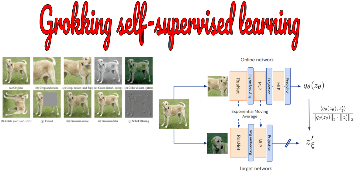
And that’s exactly where augmentations come into play. To make a positive pair, we apply 2 different stochastic transformations in the same image. To make a negative pair, we apply 2 different stochastic transformations in a different image. When a transformation is applied on an image we call it ‘view’. In the simplest case we have 2 views of an image. But this choice is kind of arbitrary. Many approaches use more than 2 views, but for educational purposes we ‘ll stick with 2!

Here is an example of some augmentations that you can apply on an image:

Examples of image augmentations. Source:SimCLR

The question is obvious. Which ones are the best for the downstream task? How do you choose augmentations and why do some work better than others?

Augmentations and their principles

In language processing, you don’t care about augmentations. The pretexts tasks are quite straightforward. The most common task for NLP is to predict missing words from a sentence.

In computer vision, we are still stuck with augmentations.

Augmentations is an indirect way to pass human prior knowledge into the model.

However, it is not straightforward how to choose these augmentations. In the famous SimCLR paper, an extensive analysis is provided to figure out which ones work:

Augmentation ablation study of SimCLR. Source

The coloured percentage is the ImageNet Top-1 accuracy after pretraining with a combination of augmentations, as shown in the non-diagonal elements. The last column reflects the average over the row.

What does this diagram mean?

Simply, that colour distortion and cropping are the key transformations to produce our views for the considered dataset.

Based on the Autoaugment paper, in datasets like SVHN, geometric transformations are more desirable, while ImageNet and CIFAR work better with colour-based transformations.

This should provide us with some sort of intuition:

Augmentation should discard the unimportant features for the downstream task. For instance, one could say that they remove the “noise” to classify an image. Whatever gets transformed, don’t pay attention to it!

Based on my short experience, here are the core principles:

Augmentations should make sense in terms of the downstream task. To understand this one consider rotation for natural images (90, 180, and 270 degrees). Even though it is used in fine-tuning or when training from scratch, you will not see it in the SSL. Why? Because it heavily changes the semantics of natural images and scenes, which brings us to the following principle.
Augmentation must maintain the image semantics (meaning). Anything that is invariant to the applied transformations must be the image schematics. We will then maximize the mutual info between the semantics between views of the same image.
Augmentation must give the model a hard time. If the model minimizes the loss too quickly it means that it’s not learning at all or that the augmentations are too easy. You can remove the crop & resize and see what happens ;).
Finally, augmentations are dependent on the dataset’s diversity and size.

Next I am referencing the augmentation pipeline for RGB images in PyTorch (for ImageNet):

import torchvision.transforms as T
import torch

img_size = 224 # your image size


color_jitter = T.ColorJitter(
   0.8 * s, 0.8 * s, 0.8 * s, 0.2 * s)

# 10% of the image usually, but be careful with small image sizes
blur = T.GaussianBlur((3, 3), (0.1, 2.0))

train_transform = torch.nn.Sequential(
   T.RandomResizedCrop(size=img_size),
   T.RandomHorizontalFlip(p=0.5),
   T.RandomApply([color_jitter], p=0.8),
   T.RandomApply([blur], p=0.5),
   T.RandomGrayscale(p=0.2),
   # global imagenet stats
   T.Normalize(mean=[0.485, 0.456, 0.406], std=[0.229, 0.224, 0.225])
)

Some papers also include image solarization, different augmentation pipelines for positives and negatives, or even different train and test augmentations. For small datasets like CIFAR blurring would be a terrible idea as the images are already small and blurry.

Before we delve into the space of features and loss functions, let’s revisit some high school math.

Logarithmic properties, and temperature softmax

You probably have seen this in high school:

log(M N)= log(M)+log(N)

log( \frac{M}{N} ) = log(M)- log(N)

p * log(M)= log(M^p)

Notice how the division in the logarithm can be written as a subtraction.

Softmax with temperature

A heavily used standardization layer before feeding the output to the loss functions is the softmax with temperature:

\operatorname{softmax}( \mathbf{x}, \tau )_{i} = \frac{exp( {x_i}/\tau) }{\sum_{1}^{K} exp({x_j}/\tau)}, \quad for \quad i=1,..,K \quad and \quad \mathbf{x} \in R^K

Intuition: The lower the temperature the sharper the model’s predictions. The closest to 0 the closest to argmax.

Argmax can be regarded as a one-hot distribution where the element with the highest value will be 1 and the other elements will be 0. As such, a low temperature (<1) discourages the predictions to collapse to a uniform distribution which is undesirable.

Counterintuitively, the self-supervised models are very sensitive to this hyperparameter! This hyperparameter is also used in the context of knowledge distillation.

Now that augmentations, logarithms and softmax are out of the way let’s see how we create a self-supervised loss between image pairs without human labels.

Loss functions: the core idea behind SSL

Let’s use the aforementioned properties. By combining the softmax with the log we have:

\operatorname{log-softmax} = \log \frac{exp( {x_i}/\tau) }{\sum_{1}^{K} exp({x_j}/\tau)}= \log(exp( {x_i}/\tau)) - \log( \sum_{1}^{K} exp\left({x_j}/ \tau \right) )

This is the core idea of self-supervised learning. The only difference is that instead of a vector we will have similarities of vector pairs.

The first term (nominator) is the “positive” pair similarity (+ in the math below). Interestingly, the second term $c$ is what we contrast the similarity on. It can be seen as a scalar.

log(exp( \operatorname{similarity^{+}} /\tau)) - c , c \in R

And since we want to minimize the similarity we need a minus sign:

-[log(exp( \operatorname{similarity^{+}} /\tau)) - c] = -log(exp( \operatorname{similarity^{+}} /\tau)) + c]

Contrastive learning: SimCLR loss function

SimCLR was the first that was proposed to learn contrastive representations.

Google AI blog: Advancing Self-Supervised and Semi-Supervised Learning with SimCLR

The loss function for a positive pair of examples (i,j) contrasted to 2N negative examples in the batch is defined as:

Loss(i,j) = -log \frac{exp( sim(x_i^{+},x_j^{+})/\tau) }{ {\sum_{k}^{\operatorname{negatives}} exp( sim(x_i^{-},x_k^{-}}/\tau)}

Admittedly, it is not that far from the context I presented so far:

-[log(exp( \operatorname{similarity^{+}} /\tau)) - c] = -log(exp( \operatorname{similarity^{+}} /\tau)) + c]

In SimCLR $c$ is computed from the negative pairs in the batch. The general idea is mean subtraction (see section below).

In the beginning, I could easily get how vector similarity can align things but how does this “pushing away” actually happens?

Well, it’s just logarithmic properties :) Or even more simply a subtraction by $c$ .

Why is this subtraction so important? Why do we care so much about subtracting something (implicit/explicit contrastive learning)?

As you probably have heard in GANs, the main problem is mode collapse! Let’s formally introduce it in the context of self-supervised learning.

Mode collapse and regularization

Mode collapse in GANs

Mode collapse refers to the generator G that fails to adequately represent the pixel-space of all the possible outputs. Instead, G selects just a few limited influential modes that correspond to noise images. In this way, D is able to easily distinguish real from fakes. Consequently, the loss of G gets highly unstable (due to exploding gradients).

Basically, G is stuck in a parameter setting where it always emits the same output.

After collapse has occurred, the discriminator learns that this output comes from the generator and the adversarial training losses diverge.

Mode collapse in self-supervised learning

Based on the DINO paper, 2 forms of mode collapse are identified in self-supervised learning [3]:

regardless of the input, the model output is uniform along all the feature dimensions, which results in random predictions. This means cross-entropy of $− log(1/c)$ for $c$ classes.
regardless of the input, the model output is dominated by one dimension, which results in zero entropy.

In both cases, the input is disregarded, and the output is the same for all the inputs.

EMA (Exponential Moving Average)

Surprisingly, the identical feature extractors don’t need to be updated with backpropagation. When this happens the gradients do not flow back to one of the networks. This operator in the literature is symbolized as stop-gradient.

The frozen model is called target or teacher while the other network is called online or student.

So how do you change the parameters without backpropagation? If the gradients remain unchanged the network will output random feature vectors.

The answer is simple: since the networks share the same architecture, we weigh the parameters of the online network with the target network. This is achieved with the so-called Exponential Moving Average (EMA).

w_{teacher} = w_{teacher}*k + (1-k) w_{student}

We fuse a tiny portion of the trained weights (less than 5%) to the frozen weights ( $k>0.95$ ).

This strategy is necessary for some SSL methods to work.

Regularization techniques

Finally, self-supervised learning needs heavy regularization. Why? Because the space of possible solutions is extremely big and there are a lot of chances of overfitting.

To encounter this problem we usually use L2 weight regularization (weight decay), LARS optimizer, learning rate warmup, learning rate decay, as well as batch normalization.

Abe Fetterman and Josh Albrecht experimented with many self-supervised approaches to draw experimental insights on the importance of implicit regularization and wrote an exceptional blog post about it. Based on their experimental analysis, they state that:

Non-contrastive learning methods like BYOL [2] often perform no better than random (mode collapse) when batch normalization is removed
The presence of batch normalization implicitly causes a form of contrastive learning by subtracting the mean based on the mini-batch statistics.

Advanced: Mean subtraction

The core difference between established SSL methods is this scalar $c$ . You can use the negative pairs from the batch. You can use an average of all the negative pairs throughout training. Or by mean subtraction from batch (batch normalization) as in BYOL. Or even subtracting the moving average features of all training batches. The latter was introduced by Facebook AI research in another type of implicit contrastive learning in DINO.

Keep in mind that there are methods that do not use negative examples from the batch to contrast representations. One of them is BYOL [2]. However, the mean subtraction in this method comes from batch normalization, which is a form of implicit contrastive learning.

Moreover, in order to cope with mode collapse BYOL introduced other tricks. First, an additional MLP called the predictor network.

Source: BYOL paper, Jean-Bastien Grill et al. 2020

The predictor breaks the symmetry between the two networks. Secondly, BYOL also enforces an Exponential Moving Average (EMA) on the target network.

In this way, the online network slowly passes its weights to the target network. This can be regarded as a mean model distillation practice. The advantage is that the noise from the student is averaged and the target network makes more stable steps. Again, the target network is not being updated with gradient descent.

The surprising results of DINO cross-entropy vs feature alignment

The minimization of similarity is directly maximizing mutual information. By applying softmax with temperature to both negatives and positives we actually pull far apart the hardest negative examples and bring together the closest positive image features.

In this sense, it was mind-blowing that an SSL method, called DINO (shown below), used cross-entropy.

Source: FAIR

Intuitively, cross-entropy after softmax (in a dimension with length K) is applied is roughly equivalent to creating some sort of clusters (soft classes). In a supervised manner, the clusters would be the image classes. Besides, given a low temperature (<1) the model has to softly assign the input in one of the K clusters, similar to fully supervised training. The number of classes/clusters is chosen arbitrarily to more than 60K. In my mind, the model extracts features based on the dataset and assigns similar features like wings of birds, faces, or dog shapes to these soft-classes.

Practical considerations

I am closing up by providing you with some ideas and tricks to make your life easier and more sane if you are experimenting with SSL methods:

Start with Adam before LARS optimizer. You can find a PyTorch implementation of LARS here.
Normalize/standardize the data at the very end of your augmentation pipeline, as the transformations may destroy the normalization. It is recommended to use the global stats of the dataset for mean/std standardization.
Start with a small model like ResNet18 and train it for at least 300 epochs.
Find a bigger dataset but from the same domain (distribution), if possible.
Have some form of evaluation during self-supervised pre-training. Examples are k-NN (k=1), or freeze the backbone and train a single linear layer for 100 epochs every couple of epochs. The latter is called linear evaluation in the literature.

Conclusion

If you learned something from this article, I would greatly appreciate sharing it with your friends & colleagues as well as on your social media. In a future article, I will attempt to run SimCLR on a small dataset like STL10 (100K unlabelled images). Finally, you can enjoy the Machine Learning Street Talk interview of can regarded Dr. Ishan Misra from Facebook AI Research to learn more about the topic:

Cited as:

@article{adaloglou2021ssl,
    title   = "Grokking self-supervised (representation) learning: how it works in computer vision and why",
    author  = "Adaloglou, Nikolas",
    journal = "https://theaisummer.com/",
    year    = "2021",
    url     = "https://theaisummer.com/self-supervised-representation-learning-computer-vision/"
  }

References

Chen, T., Kornblith, S., Norouzi, M., & Hinton, G. (2020, November). A simple framework for contrastive learning of visual representations. In International conference on machine learning (pp. 1597-1607). PMLR.
Grill, J. B., Strub, F., Altché, F., Tallec, C., Richemond, P. H., Buchatskaya, E., ... & Valko, M. (2020). Bootstrap your own latent: A new approach to self-supervised learning. arXiv preprint arXiv:2006.07733.
Caron, M., Touvron, H., Misra, I., Jégou, H., Mairal, J., Bojanowski, P., & Joulin, A. (2021). Emerging properties in self-supervised vision transformers. arXiv preprint arXiv:2104.14294.

* Disclosure: Please note that some of the links above might be affiliate links, and at no additional cost to you, we will earn a commission if you decide to make a purchase after clicking through.