If you open any introductory machine learning textbook, you will find the idea of input scaling. It is undesirable to train a model with gradient descent with non-normalized features.
In this article, we will review and understand the most common normalization methods. Different methods have been introduced for different tasks and architectures. We will attempt to associate the tasks with the methods although some approaches are quite general.
Why?
Let's start with an intuitive example to understand why we want normalization inside any model.
Imagine what will happen if the input features are lying in different ranges. Imagine that one input feature lies in the range [0,1] and another in the range [0,10000]. As a result, the model will simply ignore the first feature, given that weight is initialized in a small and close range. You don’t even need exploding gradients to occur. Yeap, that’s another problem you will face.
Similarly, we encounter the same issues inside the layers of deep neural networks. This concern is independent of the architecture (transformers, convolutional neural networks, recurrent neural networks, GANs).
If we think out of the box, any intermediate layer is conceptually the same as the input layer: it accepts features and transforms them.
To this end, we need to develop ways to train our models more effectively. Effectiveness can be evaluated in terms of training time, performance, and stability.
Below you can see a graph depicting the trends in normalization methods used by different papers through time.
 Source: papers with code
To get a better hold of all the fundamental building blocks of deep learning, we recommend the Coursera specialization.
Notations
Throughout this article, will be the batch size, while refers to the height, to the width, and to the feature channels. The greek letter μ() refers to mean and the greek letter σ() refers to standard deviation. The batch features are with a shape of [N, C, H, W]. For the referenced style image I use the symbol while for the segmentation mask I use the symbol or just mask. To recap:
Besides, we will visualize the 4D activation maps x by merging the spatial dimensions. Now we have a 3D shape that looks like this:
 An 3D vizualization of the 4D tensor
Now, we are ready!
Batch normalization (2015)
Batch Normalization (BN) normalizes the mean and standard deviation for each individual feature channel/map.
First of all, the mean and standard deviation of image features are first-order statistics. So, they relate to the global characteristics (such as the image style). In this way, we somehow blend the global characteristics. Such a strategy is effective when we want our representation to share these characteristics. This is the reason that we widely utilize BN in downstream tasks (i.e. image classification).
From a mathematical point of view, you can think of it as bringing the features of the image in the same range.
 Image by MC.AI. It show how batch norm brings the values in a compact range. Source Image
Specifically, we demand from our features to follow a Gaussian distribution with zero mean and unit variance. Mathematically, this can be expressed as:
Let’s see this operation vizually:
 An illustration of Batch Norm.
Notably, the spatial dimensions, as well as the image batch, are averaged. This way, we concentrate our features in a compact Gaussian-like space, which is usually beneficial.
In fact, γ and β correspond to the trainable parameters that result in the linear/affine transformation, which is different for all channels. Specifically γ,β are vectors with the channel dimensionality. The index c denotes the per-channel mean.
You can turn this option on or off in a deep learning framework such as PyTorch by setting affine = True/False in Python.
Advantages and disadvantages of using batch normalization
Let’s see some advantages of BN:
BN accelerates the training of deep neural networks.
For every input mini-batch we calculate different statistics. This introduces some sort of regularization. Regularization refers to any form of technique/constraint that restricts the complexity of a deep neural network during training.
Every mini-batch has a different mini-distribution. We call the change between these mini-distributions Internal Covariate Shift. BN was thought to eliminate this phenomenon. Later, Santurkar et al. [7] show that this is not exactly the case why BN works.
BN also has a beneficial effect on the gradient flow through the network. It reduces the dependence of gradients on the scale of the parameters or of their initial values. This allows us to use much higher learning rates.
In theory, BN makes it possible to use saturating nonlinearities by preventing the network from getting stuck, but we never use these kinds of activation functions.
What about disadvantages?
Inaccurate estimation of batch statistics with small batch size, which increases the model error. In tasks such as video prediction, segmentation and 3D medical image processing the batch size is usually too small. BN needs a sufficiently large batch size.
Problems when batch size is varying. Example showcases are training VS inference, pretraining VS fine tuning, backbone architecture VS head.
It is a point of discussion if the introduced regularization reduces the need for Dropout. Recent work [7] suggests that the combination of these two methods may be superior. They also provided some insights on how and why BN works. In short, they proved that BN makes the gradients more predictive. Here is the video of their video presentation (NeuIPS 2018):
Synchronized Batch Normalization (2018)
As the training scale went big, some adjustments to BN were necessary. The natural evolution of BN is Synchronized BN(Synch BN). Synchronized means that the mean and variance is not updated in each GPU separately.
Instead, in multi-worker setups, Synch BN indicates that the mean and standard-deviation are communicated across workers (GPUs, TPUs etc).
Credits for this module belong to Zhang et al. [6]. Let’s see the computation of mean and std as the calculation of these two sums:
They first calculate , and individually on each device. Then the global sums are calculated by applying the reduce parallel programing technique. The concept of reduction in parallel processing can be grasped with this video from Udacity from the parallel programming course.
Layer normalization (2016)
In ΒΝ, the statistics are computed across the batch and the spatial dims. In contrast, in Layer Normalization (LN), the statistics (mean and variance) are computed across all channels and spatial dims. Thus, the statistics are independent of the batch. This layer was initially introduced to handle vectors (mostly the RNN outputs).
We can visually comprehend this with the following figure:
 An illustration of Layer Norm.
And to be honest nobody spoke about it until the Transformers paper came out. So when dealing with vectors with batch size of , you practically have 2D tensors of shape .
Since we don’t want to be dependent on the choice of batch and it’s statistics, we normalize with the mean and variance of each vector. The math:
Generalizing into 4D feature map tensors, we can take the mean across the spatial dimension and across all channels, as illustrated below:
Instance Normalization: The Missing Ingredient for Fast Stylization (2016)
Instance Normalization (IN) is computed only across the features’ spatial dimensions. So it is independent for each channel and sample.
Literally, we just remove the sum over in the previous equation compared to BN. The figure below depicts the process:
 An illustration of Instance Norm.
Surprisingly, the affine parameters in IN can completely change the style of the output image. As opposed to BN, IN can normalize the style of each individual sample to a target style (modeled by γ and β). For this reason, training a model to transfer to a specific style is easier. Because the rest of the network can focus its learning capacity on content manipulation and local details while discarding the original global ones (i.e. style information). For completeness less check the math:
By extending this idea, by introducing a set that consists of multiple γ and β, one can design a network to model a plethora of finite styles, which is exactly the case of the so-called conditional IN [8].
But we are not only interested only in stylization, or do we?
Weight normalization (2016)
Even though it is rarely discussed we will indicate its principles. So, in Weight Normalization 2 instead of normalizing the activations x directly, we normalize the weights. Weight normalization reparametrize the weights w (vector) of any layer in the neural network in the following way:
We now have the magnitude , independent of the parameters v. Weight normalization separates the norm of the weight vector from its direction without reducing expressiveness. Basically the trainable weight vector is now v.
Adaptive Instance Normalization (2017)
Normalization and style transfer are closely related. Remember how we described IN. What if γ,β is injected from the feature statistics of another image ? In this way, we will be able to model any arbitrary style by just giving our desired feature image mean as β and variance as γ from style image .
Adaptive Instance Normalization (AdaIN) receives an input image (content) and a style input , and simply aligns the channel-wise mean and variance of x to match those of y. Mathematically:
That's all! So what can we do with just a single layer with this minor modification? Let us see!
 Architecture and results using AdaIN. Borrowed from the original work
In the upper part, you see a simple encoder-decoder network architecture with an extra layer of AdaIN for style alignment. In the lower part, you see some results of this amazing idea! If you want to play around with this idea code is available here (official).
Group normalization (2018)
Group normalization (GN) divides the channels into groups and computes the first-order statistics within each group.
As a result, GN’s computation is independent of batch sizes, and its accuracy is more stable than BN in a wide range of batch sizes. Let’s just visualize it to make the idea crystal clear:
 An illustration of group normalization
Here, I split the feature maps in 2 groups. The choice is arbitrary.
For groups=number of channels we get instance normalization, while for`groups=1 the method is reduced to layer normalization. The ugly math:
Note that G is the number of groups, which is a hyper-parameter. C/G is the number of channels per group. Thus, GN computes µ and σ along the (H, W) axes and along a group of C/G channels.
Finally, let’s see a plot of how these methods perform in the same architecture:
 Comparison using a batch size of 32 images per GPU in ImageNet. Validation error VS the numbers of training epochs is shown. The model is ResNet-50. Source: Group Normalization
The official oral paper presentation is also available from Facebook AI Research in ECCV2018:
Weight Standardization (2019)
Weight Standardization 12 is a natural evolution of Weight Normalization that we briefly discussed. Different from standard methods that focus on activations, WS considers the smoothing effects of weights. The ugly math:
All these math is a fancy way to say that we're calculating the mean and std for each output channel individually. Here is a nice way to see through the math:
 An illustration of weight standarization
In essence, WS controls the first-order statistics of the weights of each output channel individually. In this way, WS aims to normalize gradients during back-propagation.
It is theoretically and experimentally validated that it smooths the loss landscape by standardizing the weights in convolutional layers.
Theoretically, WS reduces the Lipschitz constants of the loss and the gradients. The core idea is to keep the convolutional weights in a compact space. Hence, WS smooths the loss landscape and improves training.
Remember that we observed a similar result in Wasserstein GANs. Some results from the official paper: For the record, they combined WS with Group Normalization (GN) and achieved remarkable results.
 Comparing normalization methods on ImageNet and COCO. GN+WS outperforms both BN and GN by a big margin. Source: Weight standardization paper
Later on, GN + WS have been successfully applied with tremendous success in transfer learning for NLP. For more info check Kolesnikov et al. [11]. In the following animation batch norm is coloured with red to show that by replacing the BN layers they can achieve better generalization in NLP tasks.
SPADE (2019)
We saw how we can inject a style image in the normalization module. Let’s see what we can do with segmentation maps to enforce the consistency in image synthesis. Let’s expand the idea of AdaIN a bit more. Again, we have 2 images: the segmentation map and a reference image.
How can we further constrain our model to account for the segmentation map?
Similar to BN, we will first normalize with the channel wise mean and standard deviation. But we will not rescale all the values in the channel with a scalar γ and β. Instead, we will make them tensors, that are computed with convolutions based on the segmentation mask. The math:
This step is similar to batch norm. in the last equation is the normalized value. However, since we don’t want to lose the grid structure we will not rescale all the values equally. Unlike existing normalization approaches, the new γ and β will be 3D tensors (not vectors!). Precisely, given a two-layer convolutional network with two outputs (usually called heads in the literature), we have:
We can visually illustrate this module like this:
 The SPADE layer. The image is taken from GAU-GAN paper from NVIDIA.
To see how this approach was applied to semantic image synthesis with GANs check our previous article.
Conclusion
Finally, let’s inspect all the methods comparative and try to analyze how they work.
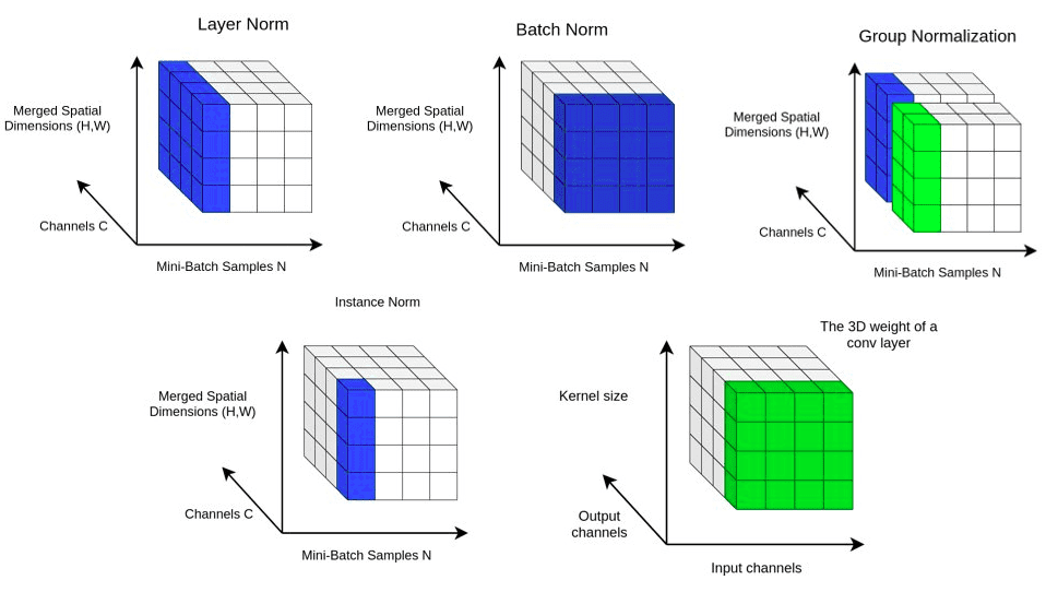
 An overview of the presented normalization methods
We presented the most famous in-layer normalization methods for training very deep models. If you liked our article, you may share it on your social media page to reach a broader audience.
Cited as:
@article{adaloglou2020normalization,title = "In-layer normalization techniques for training very deep neural networks",author = "Adaloglou, Nikolas",journal = "https://theaisummer.com/",year = "2020",url = "https://theaisummer.com/normalization/"}
References
- Ioffe, S., & Szegedy, C. (2015).Batch normalization: Accelerating deep network training by reducing internal covariate shift. arXiv preprint arXiv:1502.03167.
- Salimans, T., & Kingma, D. P. (2016). Weight normalization: A simple reparameterization to accelerate training of deep neural networks. In Advances in neural information processing systems (pp. 901-909).
- Ba, J. L., Kiros, J. R., & Hinton, G. E. (2016). Layer normalization. arXiv preprint arXiv:1607.06450.
- Ulyanov, D., Vedaldi, A., & Lempitsky, V. (2016). Instance normalization: The missing ingredient for fast stylization. arXiv preprint arXiv:1607.08022.
- Wu, Y., & He, K. (2018). Group normalization. In Proceedings of the European conference on computer vision (ECCV) (pp. 3-19).
- Zhang, H., Dana, K., Shi, J., Zhang, Z., Wang, X., Tyagi, A., & Agrawal, A. (2018). Context encoding for semantic segmentation. In Proceedings of the IEEE conference on Computer Vision and Pattern Recognition (pp. 7151-7160).
- Santurkar, S., Tsipras, D., Ilyas, A., & Madry, A. (2018). How does batch normalization help optimization?. In Advances in Neural Information Processing Systems (pp. 2483-2493).
- Dumoulin, V., Shlens, J., & Kudlur, M. (2016). A learned representation for artistic style. arXiv preprint arXiv:1610.07629.
- Park, T., Liu, M. Y., Wang, T. C., & Zhu, J. Y. (2019). Semantic image synthesis with spatially-adaptive normalization. In Proceedings of the IEEE Conference on Computer Vision and Pattern Recognition (pp. 2337-2346).
- Huang, X., & Belongie, S. (2017). Arbitrary style transfer in real-time with adaptive instance normalization. In Proceedings of the IEEE International Conference on Computer Vision (pp. 1501-1510).
- Kolesnikov, A., Beyer, L., Zhai, X., Puigcerver, J., Yung, J., Gelly, S., & Houlsby, N. (2019). Big transfer (BiT): General visual representation learning. arXiv preprint arXiv:1912.11370.
- Qiao, S., Wang, H., Liu, C., Shen, W., & Yuille, A. (2019). Weight standardization. arXiv preprint arXiv:1903.10520.

* Disclosure: Please note that some of the links above might be affiliate links, and at no additional cost to you, we will earn a commission if you decide to make a purchase after clicking through.