Understanding Maximum Likelihood Estimation in Supervised Learning

This article demystifies the ML learning modeling process under the prism of statistics. We will understand how our assumptions on the data enable us to create meaningful optimization problems. In fact, we will derive commonly used criteria such as cross-entropy in classification and mean square error in regression. Finally, I am trying to answer an interview question that I encountered: What would happen if we use MSE on binary classification?

Likelihood VS probability and probability density

To begin, let's start with a fundamental question: what is the difference between likelihood and probability? The data $x$ are connected to the possible models $\theta$ by means of a probability $P(x,\theta)$ or a probability density function (pdf) $p(x,\theta)$ .

In short, A pdf gives the probabilities of occurrence of different possible values. The pdf describes the infinitely small probability of any given value. We'll stick with the pdf notation here. For any given set of parameters $\theta$ , $p(x,\theta)$ is intended to be the probability density function of x.

The likelihood $p(x,\theta)$ is defined as the joint density of the observed data as a function of model parameters. That means, for any given x, $p(x=\operatorname{fixed},\theta)$ can be viewed as a function of $\theta$ . Thus, the likelihood function is a function of the parameters $\theta$ only, with the data held as a fixed constant.

Notations

We will consider the case were we are dealt with a set $X$ of $m$ data instances $X= \{ \textbf{x}^{(1)}, . . , \textbf{x}^{(m)} \}$ that follow the empirical training data distribution $p_{data}^{train}(\textbf{x}) = p_{data}(\textbf{x})$ , which is a good and representative sample of the unknown and broader data distribution $p_{data}^{real}(\textbf{x})$ .

The Independent and identically distributed assumption

This brings us to the most fundamental assumption of ML: Independent and Identically Distributed (IID) data (random variables). Statistical independence means that for random variables A and B, the joint distribution $P_{A,B}(a,b)$ factors into the product of their marginal distribution functions $P_{A,B}(a,b)= P_{A}(a) P_{B}(b)$ . That's how sums multi-variable joint distributions are turned into products. Note that the product can be turned into a sum by taking the $log \prod x = \sum log x$ . Since log(x) is monotonic, it's not changing the optimization problem.

Our estimator (model) will have some learnable parameters $\boldsymbol{\theta}$ that make another probability distribution $p_{model}(\textbf{x}, \boldsymbol{\theta})$ . Ideally, $p_{model}(\textbf{x}, \boldsymbol{\theta}) \approx p_{data}(\textbf{x})$ .

The essence of ML is to pick a good initial model that exploits the assumptions and the structure of the data. Less literally, a model with a decent inductive bias. As the parameters are iteratively optimized, $p_{model}(\textbf{x}, \boldsymbol{\theta})$ gets closer to $p_{data}(\textbf{x})$ .

In neural networks, because the iterations happen in a mini-batch fashion instead of the whole dataset, $m$ will be the mini-batch size.

Maximum Likelihood Estimation (MLE)

Maximum Likelihood Estimation (MLE) is simply a common principled method with which we can derive good estimators, hence, picking $\boldsymbol{\theta}$ such that it fits the data.

To disentangle this concept, let's observe the formula in the most intuitive form:

\boldsymbol{\theta}_{\mathrm{MLE}}= \underset{\operatorname{params}}{\arg \max } \operatorname{p}_{\operatorname{model}}( \operatorname{output} | {\operatorname{inputs}},\operatorname{params})

The optimization problem is maximizing the likelihood of the given data. Outputs are the conditions in the probability world. Unconditional MLE means we have no conditioning on the outputs, so no labels.

\begin{aligned} \boldsymbol{\theta}_{\mathrm{MLE}} &=\underset{\boldsymbol{\theta}}{\arg \max } \operatorname{p}_{\text {model }}({X} , \boldsymbol{\theta}), \\ &=\underset{\boldsymbol{\theta}}{\arg \max } \prod_{i=1}^{m} \operatorname{p}_{\text {model }}\left(\boldsymbol{x}^{(i)} , \boldsymbol{\theta}\right) . \end{aligned}

In a supervised ML context, the condition would simply be the data labels.

\boldsymbol{\theta}_{\mathrm{ML}}=\underset{\boldsymbol{\theta}}{\arg \max } \sum_{i=1}^{m} \log p_{model}\left(\boldsymbol{y}^{(i)} \mid \boldsymbol{x}^{(i)} , \boldsymbol{\theta}\right)

Quantifying distribution closeness: KL-div

One way to interpret MLE is to view it as minimizing the "closeness" between the training data distribution $p_{data}(\textbf{x})$ and the model distribution $p_{model}(\textbf{x}, \boldsymbol{\theta})$ . The best way to quantify this "closeness" between distributions is the KL divergence, defined as:

\begin{gathered} D_{K L}( p_{data} \| p_{model})=E_{x\sim p_{data}} [ \log \frac{p_{data}(\textbf{x})}{p_{model}(\textbf{x}, \boldsymbol{\theta})}] = \\ E_{x\sim p_{data}} [ \log p_{data}(\textbf{x}) - \log p_{model}(\textbf{x}, \boldsymbol{\theta})], \end{gathered}

where $E$ denotes the expectation over all possible training data. In general, the expected value $E$ is a weighted average of all possible outcomes. We will replace the expectation with a sum, whilst multiplying each term with its possible "weight" of happening, that is $p_{data}$ .

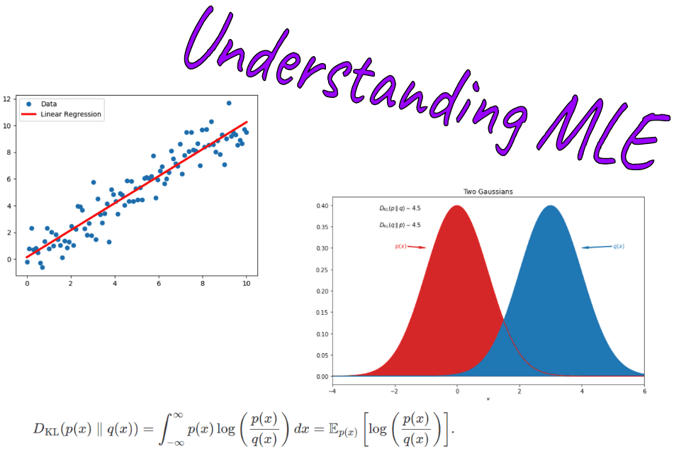
Illustration of the relative entropy for two normal distributions. The typical asymmetry is clearly visible. By Mundhenk at English Wikipedia, CC BY-SA 3.0

Notice that I intentionally avoided using the term distance. Why? Because a distance function is defined to be symmetric. KL-div, on the other hand, is asymmetric meaning $D_{K L}( p_{data} \| p_{model}) \neq D_{K L}(p_{model} \| p_{data} )$ .

Source: Datumorphism

Intuitively, you can think of $p_{data}$ as a static "source" of information that sends (passes) batches of data to $p_{model}$ , the "receiver". Since information is passed one way only, that is from $p_{data}$ to $p_{model}$ , it would make no sense to calculate the distance with $p_{model}$ as the reference source. You can practically observe this nonsense by swapping the target and the model prediction in the cross-entropy or KL-div loss function in your code.

By replacing the expectation $E$ with our lovely sum:

\begin{gathered} D_{K L}(p_{data} \| p_{model})=\sum_{x=1}^{N} p_{data}(\textbf{x}) \log \frac{p_{data}(\textbf{x})}{p_{model}(\textbf{x}, \boldsymbol{\theta})} \\ =\sum_{x=1}^{N} p_{data}(\textbf{x})[\log p_{data}(\textbf{x})-\log p_{model}(\textbf{x}, \boldsymbol{\theta})] \end{gathered}

When we minimize the KL divergence with respect to the parameters of our estimator, $\log p_{data}(\textbf{x})$ gets out of the way, which brings us to:

\nabla_{\theta} D_{K L}(p_{data} \| p_{model}) = - \sum_{x=1}^{N} p_{data}(\textbf{x}) \log p_{model}(\textbf{x}, \boldsymbol{\theta}).

In other words, minimizing KL-div is mathematically equivalent to minimizing cross-entropy ( $H(P, Q)=-\sum_{x} P(x) \log Q(x)$ ) :

\begin{aligned} H\left(p_{data}, p_{model}\right) &=H(p_{data})+D_{K L}\left(p_{data} \| p_{model}\right) \\ \nabla_{\theta} H\left(p_{data}, p_{model}\right) &=\nabla_{\theta}\left(H(p_{data})+D_{K L}\left(p_{data} \| p_{model}\right)\right) \\ &=\nabla_{\theta} D_{K L}\left(p_{data} \| p_{model}\right) \end{aligned}

The optimal parameters $\boldsymbol{\theta}$ will, in principle, be the same. Even though the optimization landscape would be different (as defined by the objective functions), maximizing the likelihood is equivalent to minimizing the KL divergence. In this case, the entropy of the data $H(p_{data})$ will shift the landscape, while a scalar multiplication would scale the optimization landscape. Sometimes I find it helpful to imagine the landscape as descending a mountain. Practically, both are framed as minimizing an objective cost function.

From the statistical point of view, it's more of bringing the distributions close so KL-div. From the aspect of information theory, cross-entropy might make more sense to you.

MLE in Linear regression

Let's consider linear regression. Imagine that each single prediction $\hat{y}$ produces a "conditional" distribution $p_{model}(\hat{y} | \textbf{x})$ , given a sufficiently large train set. The goal of the learning algorithm is again to match the distribution $p_{data}(y | \textbf{x})$ .

Source

Now we need an assumption. We hypothesize the neural network or any estimator $f$ as $\hat{y}=f(\textbf{x} , \theta)$ . The estimator approximates the mean of the normal distribution ( $N(\mu,\sigma)$ ) the we choose to parametrize $p_{data}$ . Specifically, in the simplest case of linear regression we have $\mu = \boldsymbol{\theta}^T \mathbf{x}$ . We also assume a fixed standard deviation $\sigma$ of the normal distribution. These assumptions immediately causes MLE to become Mean Squared Error (MSE) optimization. Let's see how.

\begin{aligned} & \hat{y}=f(\textbf{x} , \boldsymbol{\theta}) \\ y & \sim \mathcal{N}\left(y , \mu=\hat{y}, \sigma^{2}\right) \\ p(y \mid \textbf{x} , \boldsymbol{\theta}) &=\frac{1}{\sigma \sqrt{2 \pi}} \exp \left(\frac{-(y-\hat{y})^{2}}{2 \sigma^{2}}\right) \end{aligned}

In terms of log-likelihood we can form a loss function:

\begin{aligned} L &=\sum_{i=1}^{m} \log p(y \mid \textbf{x} , \boldsymbol{\theta}) \\ &=\sum_{i=1}^{m} \log \frac{1}{\sigma \sqrt{2 \pi}} \exp \left(\frac{-\left(\hat{y}^{(i)}-y^{(i)}\right)^{2}}{2 \sigma^{2}}\right) \\ &=\sum_{i=1}^{m}-\log (\sigma \sqrt{2 \pi})-\log \exp \left(\frac{(\hat{y}^{(i)}-y^{{(i)}} )^{2}.}{2 \sigma^{2}}\right) \\ &=\sum_{i=1}^{m}-\log (\sigma)-\frac{1}{2} \log (2 \pi)-\frac{(\hat{y}^{(i)}-y^{{(i)}})^{2}}{2 \sigma^{2}} \\ &=-m \log (\sigma)-\frac{m}{2} \log (2 \pi)-\sum_{i=1}^{m} \frac{\left(\hat{y}^{(i)}-y^{{(i)}}\right)^{2}}{2 \sigma^{2}} \\ \end{aligned}

By taking the partial derivative with respect to the parameters, we get the desired MSE.

\begin{aligned} \nabla_{\theta} L &=-\nabla_{\theta} \sum_{i=1}^{m} \frac{\left\|\hat{y}^{(i)}-y^{(i)}\right\|^{2}}{2 \sigma^{2}} \\ &=-m \log (\sigma)-\frac{m}{2} \log (2 \pi)-\sum_{i=1}^{m} \frac{\left\|\hat{y}^{(i)}-y^{(i)}\right\|^{2}}{2 \sigma^{2}} \\ &=-m \log (\sigma)-\frac{m}{2} \log (2 \pi)- \frac{m}{2 \sigma^{2}} MSE \end{aligned}

Since $\operatorname{MSE}=\frac{1}{m} \sum_{i=1}^{m}\left\|\hat{y}^{(i)}-y^{(i)}\right\|^{2}$

MLE in supervised classification

In linear regression, we parametrized $p_{model}(y | \mathbf{x}, \boldsymbol{\theta})$ as a normal distribution. More precisely, we parametrized the mean to be $\mu = \boldsymbol{\theta}^T \mathbf{x}$ .

It is possible to convert linear regression to a classiﬁcation problem. All we need to do is encode the ground truth as a one-hot vector:

p_{data}\left(y \mid \textbf{x}_{i}\right)= \begin{cases}1 & \text { if } y=y_{i} \\ 0 & \text { otherwise }\end{cases} ,

where $i$ refer to a single data instance.

\begin{aligned} H_{i}\left(p_{data}, p_{model}\right) &=-\sum_{y \in Y} p_{data}\left(y \mid \textbf{x}_{i}\right) \log p_{model}\left(y \mid \textbf{x}_{i}\right) \\ &=-\log p_{model}\left(y_{i} \mid \textbf{x}_{i}\right) \end{aligned}

For simplicity let's consider the binary case of two labels, 0 and 1.

\begin{aligned} L &=\sum_{i=1}^{n} H_{i}\left(p_{data}, p_{model}\right) \\ &=\sum_{i=1}^{n}-\log p_{model}\left(y_{i} \mid \textbf{x}_{i}\right) \\ &=-\sum_{i=1}^{n} \log p_{model}\left(y_{i} \mid \textbf{x}_{i}\right) \end{aligned}

\begin{aligned} =\underset{\boldsymbol{\theta}}{\arg \min } L &= \underset{\boldsymbol{\theta}}{\arg \min } -\sum_{i=1}^{n} \log p_{model}\left(y_{i} \mid \textbf{x}_{i}\right) \end{aligned}

This is in line with our definition of conditional MLE:

\boldsymbol{\theta}_{\mathrm{ML}}=\underset{\boldsymbol{\theta}}{\arg \max } \sum_{i=1}^{m} \log p_{model}\left(\boldsymbol{y}^{(i)} \mid \boldsymbol{x}^{(i)} , \boldsymbol{\theta}\right)

Broadly speaking, MLE can be applied to most (supervised) learning problems,

by specifying a parametric family of (conditional) probability distributions.

Another way to achieve this in a binary classification problem would be to take the scalar output $y$ of the linear layer and pass it from a sigmoid function. The output will be in the range [0,1] and we define this as the probability of $p(y = 1 | \mathbf{x}, \boldsymbol{\theta})$ .

p(y = 1 | \mathbf{x}, \boldsymbol{\theta}) = \sigma( \boldsymbol{\theta}^T \mathbf{x}) = \operatorname{sigmoid}( \boldsymbol{\theta}^T \mathbf{x}) \in [0,1]

Consequently, $p(y = 0 | \mathbf{x}, \boldsymbol{\theta}) = 1 - p(y = 1 | \mathbf{x}, \boldsymbol{\theta})$ . In this case binary-cross entropy is practically used. No closed form solution exist here, one can approximate it with gradient descend. For reference, this approach is surprisingly known as ""logistic regression".

Bonus: What would happen if we use MSE on binary classification?

So far I presented the basics. This is a bonus question that I was asked during an ML interview: What if we use MSE on binary classification?

When $\hat{y}^{(i)}=0$ :

\operatorname{MSE}=\frac{1}{m} \sum_{i=1}^{m}\left\|-y^{(i)}\right\|^{2}= \frac{1}{m} \sum_{i=1}^{m}\left\|-\sigma( \boldsymbol{\theta}^T \mathbf{x}) \right\|^{2} = \frac{1}{m} \sum_{i=1}^{m}\left\|\sigma( \boldsymbol{\theta}^T \mathbf{x}) \right\|^{2}

When $\hat{y}^{(i)}=1$ :

\operatorname{MSE}=\frac{1}{m} \sum_{i=1}^{m}\left\|1 -y^{(i)}\right\|^{2}= \frac{1}{m} \sum_{i=1}^{m}\left\|1 - \sigma( \boldsymbol{\theta}^T \mathbf{x}) \right\|^{2}

One intuitive way to guess what's happening without diving into the math is this one: in the beginning of training the network will output something very close to 0.5, which gives roughly the same signal for both classes. Below is a more principled method proposed after the initial release of the article by Jonas Maison.

Proposed demonstration by Jonas Maison

Let's assume that we have a simple neural network with weights $\theta$ such as $z=\theta^\intercal x$ , and outputs $\hat{y}=\sigma(z)$ with a sigmoid activation.

\frac{\partial L}{\partial \theta}=\frac{\partial L}{\partial \hat{y}}\frac{\partial \hat{y}}{\partial z}\frac{\partial z}{\partial \theta}

MSE Loss

L(y, \hat{y}) = \frac{1}{2}(y-\hat{y})^2

\frac{\partial L}{\partial \theta}=-(y-\hat{y})\sigma(z)(1-\sigma(z))x

\frac{\partial L}{\partial \theta}=-(y-\hat{y})\hat{y}(1-\hat{y})x

$\sigma(z)(1-\sigma(z))$ makes the gradient vanish if $\sigma(z)$ is close to 0 or 1. Thus, the neural net can't train.

Binary Cross Entropy (BCE) Loss

L(y, \hat{y}) = -ylog(\hat{y})-(1-y)log(1-\hat{y})

For $y=0$ :

\frac{\partial L}{\partial \theta}=\frac{1-y}{1-\hat{y}}\sigma(z)(1-\sigma(z))x

\frac{\partial L}{\partial \theta}=\frac{1-y}{1-\hat{y}}\hat{y}(1-\hat{y})x

\frac{\partial L}{\partial \theta}=(1-y)(\hat{y})x

\frac{\partial L}{\partial \theta}=\hat{y}x

If the network is right, $\hat{y}=0$ , the gradient is null.

For $y=1$ :

\frac{\partial L}{\partial \theta}=-\frac{y}{\hat{y}}\sigma(z)(1-\sigma(z))x

\frac{\partial L}{\partial \theta}=-\frac{y}{\hat{y}}\hat{y}(1-\hat{y})x

\frac{\partial L}{\partial \theta}=-y(1-\hat{y})x

\frac{\partial L}{\partial \theta}=-(1-\hat{y})x

If the network is right, $\hat{y}=1$ , the gradient is null.

Conclusion and References

This short analysis explains why we blindly choose our objective functions to minimize such as cross-entropy. MLE is a principled way to define an optimization problem and I find it a common discussion topic to back up design choices during interviews.

Deep learning - Information theory and Maximum likelihood by Jonathan Hui.
Cross-Entropy, KL Divergence, and Maximum Likelihood Estimation by Lei Mao.
Chapter 5, Machine Learning Basics, Deep learning book by Ian Goodfellow and Yoshua Bengio and Aaron Courville

If you like our content consider supporting us, by any possible means. It would be massively appreciated.

* Disclosure: Please note that some of the links above might be affiliate links, and at no additional cost to you, we will earn a commission if you decide to make a purchase after clicking through.