Deep learning in medical imaging - 3D medical image segmentation with PyTorch

Deep learning and medical imaging

The rise of deep networks in the field of computer vision provided state-of-the-art solutions in problems that classical image processing techniques performed poorly. In the generalized task of image recognition, which includes problems such as object detection, image classification, and segmentation, activity recognition, optical flow and pose estimation, we can easily claim that DNN (Deep Neural Networks) have achieved superior performance.

Along with this rise in computer vision, there has been a lot of interest in the application in the field of medical imaging. Even though medical imaging data are not so easy to obtain, DNN’s seem to be an ideal candidate to model such complex and high dimensional data.

Recently, Imperial College of London launched a course on COVID-19. A lot of researches have already attempted to automatically detect COVID-19 through deep networks from 3D CT scans. Nevertheless, the application-specific data are still not available it is clear that AI will hugely impact the evolution of medicine through medical imaging.

As we will see a medical image is often three or four-dimensional. Another reason that this field attracts a lot of attention is its direct impact on human lives. Medical errors are the third-leading cause of death, after heart disease and cancer in the USA. Consequently, it is obvious that the first three causes of human deaths are related to medical imaging. That’s why it is estimated that AI and deep learning in medical imaging will create a brand new market of more than a billion dollars by 2023.

This work serves as an intersection of these two worlds: Deep neural networks and medical imaging. In this post, we will tackle the problem of medical image segmentation, focused on magnetic resonance images, which is one of the most popular tasks, because it is the task with the most well-structured datasets that someone can get access to. Since online medical data collection is not as straightforward as it may sound; a collection of links to start your journey is provided at the end of the article.

This article presents some preliminary results of an under development open-source library, called MedicalZoo that can be found here.

To dive deeper into how AI is used in Medicine, you can’t go wrong with the AI for Medicine there is out there! Use the discount code aisummer35 to get an exclusive 35% discount from your favorite AI blog.

The need for 3D Medical image segmentation

3D Volumetric image segmentation in medical images is mandatory for diagnosis, monitoring, and treatment planning. We will just use magnetic resonance images (MRI). Manual practices require anatomical knowledge and they are expensive and time-consuming. Plus, they can be inaccurate due to the human factor. Nevertheless, automated volume segmentation can save physicians time and provide an accurate reproducible solution for further analysis.

We will start by describing the fundamentals of MR Imaging because it is crucial to understand your input data to train a deep architecture. Then, we provide the reader with an overview of 3D-UNET that can be efficiently used for this task.

Medical images and MRI

Medical imaging seeks to reveal internal structures hidden by the skin and bones, as well as to diagnose and treat diseases. Medical magnetic resonance (MR) imaging uses the signal from the nuclei of hydrogen atoms for image generation. In the case of hydrogen nuclei: when it is exposed to an external magnetic field, denoted as B0, the magnetic moments, or spins, align with the direction of the field like compass needles.

All of the constant magnetization is rotated into another plane by an additional radio-frequency pulse that is strong enough and applied long enough to tip the magnetization. Immediately after excitation, the magnetization rotates in the other plane. The rotating magnetization gives rise to the MR signal in the receiver coil. However, the MR signal rapidly fades due to two independent processes that reduce magnetization and thus cause a return to the stable state present before excitation that produce the so-called T1 images and T2 magnetic resonance images. T1 relaxation is related to the nuclei that excess energy to their surroundings, while T2 relaxation refers to the phenomenon of the individual magnetization vectors that begin to cancel each other. The aforementioned phenomena are completely independent. As a consequence, different intensities represent different tissues, as illustrated below:

Image taken from this book.

3D Medical image representation

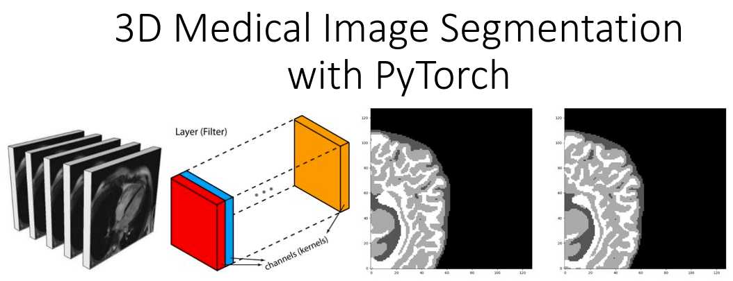
Since medical images represent 3D structure, one way that you can deal with them is by using slices of the 3D volume and perform regular 2D sliding convolutions, as illustrated in the figure below. Let’s suppose that the red rectangle is an image 5x5 patch that can be represented with a matrix that contains the intensity values. The voxel intensities and the kernel are convolved with a 3x3 convolution kernel, as shown in the Figure below. In the same pattern, the kernel is slided across the whole 2D grid (medical image slice) and every time we perform cross-correlation. The result of a convolved 5x5 patch is stored in a 3x3 matrix (no padding for illustration purposes) and is propagated in the next layer of the network.

Alternatively, you can represent them similar to an output of an intermediate layer. In deep architectures, we usually have multiple feature maps, which is practically a 3D tensor. If there is a reason to believe that there are patterns among the additional dimension it is optimal to perform 3D sliding convolution. This is the case in medical images. Similar to the 2D convolutions, which encode spatial relationships of objects in a 2D domain, 3D convolutions can describe the spatial relationships of objects in the 3D space. Since 2D representation is sub-optimal for medical images, we will opt out to use 3D convolutional networks in this post.

Medical image slices can be seen as multiple feature maps of an intermediate layer, with the difference that they have a strong spatial relationship

Model: 3D-Unet

For our example, we will use the well-accepted 3D U-shaped network. The latter (code) expands the successive idea of a symmetrical u-shaped 2D Unet network that yields impressive results in RGB-related tasks, such as semantic segmentation. The model has an encoder(contracting path) and a decoder (synthesis path) path each with four resolution steps. In the encoder path, each layer contains two 3 ×3 ×3 convolutions each followed by a rectiﬁed linear unit (ReLu), and then a 2 ×2 ×2 max pooling with strides of two in each dimension. In the decoder path, each layer consists of a transpose convolution of 2 ×2 ×2 by strides of two in each dimension, followed by two 3 ×3 ×3 convolutions each followed by a ReLu. Shortcut skip connections from layers of equal resolution in the analysis path provide the essential high-resolution features to the synthesis path. In the last layer, a 1×1×1 convolution reduces the number of output channels to the number of labels. Bottlenecks are avoided by doubling the number of channels already before max pooling. 3D batch normalization is introduced before each ReLU. Each batch is normalized during training with its mean and standard deviation and global statistics are updated using these values. This is followed by a layer to learn scale and bias explicitly. The Fig. below illustrates the network architecture.

Network architecture taken from the 3D Unet original paper

Loss function: Dice Loss

Due to the inherent task imbalance, cross-entropy cannot always provide good solutions for this task. Specifically, cross-entropy loss examines each pixel individually, comparing the class predictions (depth-wise pixel vector) to our one-hot encoded target vector. Because the cross-entropy loss evaluates the class predictions for each pixel vector individually and then averages over all pixels, we are essentially asserting equal learning to each pixel in the image. This can be a problem if your various classes have unbalanced representation in the image, as the most prevalent class can dominate training.

The 4 classes that we will try to distinguish in brain MRI have different frequencies in an image (i.e. air has way more instances than the other tissues). That’s why the dice loss metric is adopted. It is based on the Dice coefficient, which is essentially a measure of overlap between two samples. This measure ranges from 0 to 1 where a Dice coefficient of 1 denotes perfect and complete overlap. Dice loss was originally developed for binary classification, but it can be generalized to work with multiple classes. Feel free to use our multi-class implementationof Dice loss.

Medical imaging data

Deep architectures requiring a large number of training samples before they can produce anything useful generalized representation and labeled training data are typically both expensive and difficult to produce. That’s why we see every day new techniques that use generative learning to produce more and more medical imaging data. Besides, the training data must be representative of the data the network will meet in the future. If the training samples are drawn from a data distribution that is different from the one would meet in the real world, then the network's generalization performance will be lower than expected.

Since we are focusing on brain MRI automatic segmentation, it is important to briefly describe the basic structures of the brain that DNN’s are trying to distinguish a) White matter(WM), b) Grey matter(GM), c) Cerebrospinal fluid(CSF). The following figure illustrates the segmented tissues in brain MRI slice.

Borrowed from I-seg 2017 medical data MICCAI challenge

I-Seg medical image data challenge 2017

Accurate segmentation of infant brain MRI images into white matter (WM), gray matter (GM), and cerebrospinal fluid (CSF) in this critical period are of fundamental importance in studying both normal and abnormal early brain development. The first year of life is the most dynamic phase of the postnatal human brain development, along with rapid tissue growth and development of a wide range of cognitive and motor functions. This early period is critical in many neurodevelopmental and neuropsychiatric disorders, such as schizophrenia and autism. More and more attention has been paid to this critical period.

This dataset aims to promote automatic segmentation algorithms on 6-month infant brain MRI. This challenge was carried out in conjunction with MICCAI 2017, with a total of 21 international teams. The dataset contains 10 densely annotated images from experts and 13 imaging for testing. Test labels are not provided, and you can only see your score after uploading the results on the official website. For each subject, there is a T1 weighted and T2 weighted image.

The first subject will be used for testing. The original MR volumes are of size 256x192x144. In 3D-Unet the sampled sub-volumes that were used are of size 128x128x64. The training dataset that was generated consisted of 500 sub-volumes. For the validation set, 10 random samples from one subject were used.

Medical Zoo Pytorch

WHY: Our goal is to implement an open-source medical image segmentation library of state of the art 3D deep neural networks in PyTorch along with data loaders of the most common medical datasets. The first stable release of our repository is expected to be published soon.

We strongly believe in open and reproducible deep learning research. In order to reproduce our results, the code and materials of this work are available in this repository. This project started as a MSc Thesis and is currently under further development.

Putting it all together

Implementation Details

We used PyTorch framework, which is considered the most widely accepted deep learning research tool. Stochastic gradient descend with a single batch size with learning rate 1e-3 and weight decay 1e-8 was used for all experiments. We provided tests in our repository that you can easily reproduce our results so that you can use the code, models, and data loaders.

Recently we added Tensorboard visualization with Pytorch. This amazing feature keeps your sanity in-place and lets you track the training process of your model. Below you can see an example of keeping the training stats, dice coeff. and loss as well as the per class-score to understand the model behavior.

Code

Let’s put all the described modules together to set up an experiment in a short script (for illustration purposes) with MedicalZoo.

# Python libraries
import argparse
import os

# Lib files
import lib.medloaders as medical_loaders
import lib.medzoo as medzoo
import lib.train as train
import lib.utils as utils
from lib.losses3D import DiceLoss

def main():
    args = get_arguments()
    utils.make_dirs(args.save)

    training_generator, val_generator, full_volume, affine = medical_loaders.generate_datasets(args,
                                                                                               path='.././datasets')
    model, optimizer = medzoo.create_model(args)
    criterion = DiceLoss(classes=args.classes)

    if args.cuda:
        model = model.cuda()
        print("Model transferred in GPU.....")

    trainer = train.Trainer(args, model, criterion, optimizer, train_data_loader=training_generator,
                            valid_data_loader=val_generator, lr_scheduler=None)
    print("START TRAINING...")
    trainer.training()


def get_arguments():
    parser = argparse.ArgumentParser()
    parser.add_argument('--batchSz', type=int, default=4)
    parser.add_argument('--dataset_name', type=str, default="iseg2017")
    parser.add_argument('--dim', nargs="+", type=int, default=(64, 64, 64))
    parser.add_argument('--nEpochs', type=int, default=200)
    parser.add_argument('--classes', type=int, default=4)
    parser.add_argument('--samples_train', type=int, default=1024)
    parser.add_argument('--samples_val', type=int, default=128)
    parser.add_argument('--inChannels', type=int, default=2)
    parser.add_argument('--inModalities', type=int, default=2)
    parser.add_argument('--threshold', default=0.1, type=float)
    parser.add_argument('--terminal_show_freq', default=50)
    parser.add_argument('--augmentation', action='store_true', default=False)
    parser.add_argument('--normalization', default='full_volume_mean', type=str,
                        help='Tensor normalization: options ,max_min,',
                        choices=('max_min', 'full_volume_mean', 'brats', 'max', 'mean'))
    parser.add_argument('--split', default=0.8, type=float, help='Select percentage of training data(default: 0.8)')
    parser.add_argument('--lr', default=1e-2, type=float,
                        help='learning rate (default: 1e-3)')
    parser.add_argument('--cuda', action='store_true', default=True)
    parser.add_argument('--loadData', default=True)
    parser.add_argument('--resume', default='', type=str, metavar='PATH',
                        help='path to latest checkpoint (default: none)')
    parser.add_argument('--model', type=str, default='VNET',
                        choices=('VNET', 'VNET2', 'UNET3D', 'DENSENET1', 'DENSENET2', 'DENSENET3', 'HYPERDENSENET'))
    parser.add_argument('--opt', type=str, default='sgd',
                        choices=('sgd', 'adam', 'rmsprop'))
    parser.add_argument('--log_dir', type=str,
                        default='../runs/')

    args = parser.parse_args()

    args.save = '../saved_models/' + args.model + '_checkpoints/' + args.model + '_{}_{}_'.format(
        utils.datestr(), args.dataset_name)
    return args


if __name__ == '__main__':
    main()

Experimental results

Below you can see the training and validation dice loss curve of the model. It is important to monitor your model performance and tune the parameters to get such a smooth training curve. It is easy to understand the efficiency of this model.

Surprisingly, the model reaches a dice coeff score of roughly 93% in the validation set of sub-volumes. Last but not least, let’s see some visualisation predictions from 3D-Unet in the validation set. We present only a representative slice here, although the prediction is a 3D-volume. By taking multiple sub-volumes of the MRI, one can combine them to form a full 3D MRI segmentation. Note that, the fact that we use sub-volumes sampling serves as data augmentation.

Unnormalized last layer pre-activation from trained 3D-Unet. The network learns highly semantic task-relevant content that corresponds to brain structures similar to the input.

Our prediction VS Ground truth. Which prediction do you think is the ground truth? Look closely before you decide! As a note, we only present the median axial slice here, but the prediction is a 3D volume. One can observe that the network predicts air voxels perfectly, while it has difficulty in distinguishing the tissue boundaries. But, let’s check again to find out the real one!

Now, I am sure you can distinguish the ground truth. If you are not sure, check the end of the article :)

Recently we also added Tensorboard vizualization with Pytorch. This amazing feature keeps your sanity in-place and let’s you track the training process of your model. Below you can see an example of keeping the training stats, dice coefficient and loss as well as the per class-score to understand the model behaviour.

It is obvious that the different tissues have different accuracies, even from the start of the training. For example, look at air voxels in the validation set that start from a high value because it is the most dominant class of an imbalanced dataset. On the other hand, grey matter starts from the lowest value, because it is the most difficult to distinguish and with the less training instances.

Conclusion

This post serves partly as an illustration of some of the features of MedicalZoo Pytorch library that is developed by our team. Deep learning models will provide society with immerse medical image solutions.

In this article, we reviewed the basic concepts of medical imaging and MRI, as well as how they can be represented and used in a deep learning architecture. Then, we described an efficient widely accepted 3D architecture (Unet) and the dice loss function to handle class imbalance. Finally, we combined all the above-described features and used the library scripts to provide the preliminary results of our experimental analysis in brain MRI. The results demonstrate the efficiency of 3D architectures and the potential of deep learning in medical image analysis.

Finally, there are unlimited opportunities to improve current medical image solutions for a plethora of problems, so stay updated for more biomedical imaging posts with Python and our beloved Pytorch. To dive deeper into how AI is used in Medicine, you can't go wrong with this online course by Coursera: AI for Medicine

Stay tuned for more medical imaging AI summer tutorials.

Appendix - Where to find medical imaging data

If you reached this point and understood the main points of this article, I am really happy. That’s why I will reveal that the ground truth image is the left one 😊. Unfortunately, medical image data cannot be shared or used for commercial reasons. Please feel free to navigate in the following links in order to download the data. Feel free to share with us your own exciting machine learning solutions.

References:

Adaloglou Nikolas, Evangelos Dermatas (2019). Deep learning in medical image analysis: a comparative analysis of multi-modal brain-MRI segmentation with 3D deep neural networks

* Disclosure: Please note that some of the links above might be affiliate links, and at no additional cost to you, we will earn a commission if you decide to make a purchase after clicking through.