How Positional Embeddings work in Self-Attention (code in Pytorch)

If you are reading transformer papers, you may have noticed Positional Embeddings (PE). They may seem reasonable. However, when you try to implement them, it becomes really confusing!

The answer is simple: if you want to implement transformer-related papers, it is very important to get a good grasp of positional embeddings.

It turns out that sinusoidal positional encodings are not enough for computer vision problems. Images are highly structured and we want to incorporate some strong sense of position (order) inside the multi-head self-attention (MHSA) block.

To this end, I will introduce some theory as well as my re-implementation of positional embeddings.

The code contains einsum operations. Read my past article if you are not comfortable with it. The code is also available.

Positional encodings vs positional embeddings

In the vanilla transformer, positional encodings are added before the first MHSA block model. Let’s start by clarifying this: positional embeddings are not related to the sinusoidal positional encodings. It’s highly similar to word or patch embeddings, but here we embed the position.

Each position of the sequence will be mapped to a trainable vector of size $dim$

Moreover, positional embeddings are trainable as opposed to encodings that are fixed.

Here is a rough illustration of how this works:

# initialization
pos_emb1D = torch.nn.Parameter(torch.randn(max_seq_tokens, dim))
# during forward pass
input_to_transformer_mhsa = input_embedding + pos_emb1D[:current_seq_tokens, :]

out = transformer(input_to_transformer_mhsa)

By now you are probably wondering what PE learn. Me too!

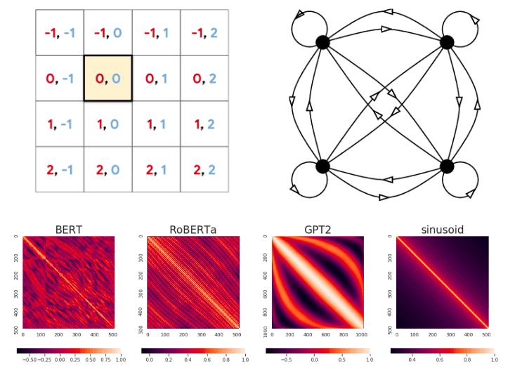
Here is a beautiful illustration of the positional embeddings from different NLP models from Wang et Chen 2020 [1]:

Position-wise similarity of multiple position embeddings. Image from Wang et Chen 2020

In short, they visualized the position-wise similarity of different position embeddings. Brighter in the figures denotes higher similarity. Note that larger models such as GPT2 process more tokens (horizontal and vertical axis).

However, we have many reasons to enforce this idea inside MHSA.

How Positional Embeddings emerged inside MHSA

If the PE are not inside the MHSA block, they have to be added to the input representation, as we saw. The main concern is that they will only be available once in the beginning.

The well-known MHSA mechanism encodes no positional information, which makes it permutation equivariant. The latter limits its representational power for computer vision tasks.

Why?

Because images are highly-structured data.

So it would make more sense to come up with MHSA modules that respect the order (structure) that LSTM’s enjoy for free.

PE provides a solution to this problem. To intuitively understand it we have to delve into self-attention.

The weights of self-attention model the input sequence as a fully-connected directed graph.

A fully-connected graph with four vertices and sixteen directed bonds..Image from Gregory Berkolaiko. Source: ResearchGate

You can think of each attention weight $\epsilon_{ij}$ as an arrow.

\epsilon_{ij} =\frac{x_i W^Q(x_jW^K)^T}{\sqrt{d}}

The index $i$ will indicate the query and the index $j$ the key and the value.

You are probably wondering why $i$ indexes the query and $j$ indexes the keys and values. Here is a nice illustration:

Source: Ramachandran et al. Stand-Alone Self-Attention in Vision Models

Each individual output element comes a single query element indexed by $i$ . The query element $q_i$ will be associated to all the elements of the input sequences, indeed by $j$ .

PE aim to inject some positional information in this computation. So we consider the positions $p_{ij} \in R^d$ of the Keys with respect to the query element.

\epsilon_{ij} =\frac{x_i W^Q(x_jW^K)^T + x_i W^Q(p_{ij}^K)^T}{\sqrt{d}}

The added $x_i W^Q(p_{ij}^K)^T$ term represents the distance of the query element to a particular sequence position.

A great thing with PE is that we can have shared representations across heads, introducing minimal overhead. For a sequence of length $n$ and $h$ attention heads with head dimension $d$ , this reduces the space complexity from $O(h n^2 d )$ to $O(n^2 d)$ .

Let’s further divide Positional Embeddings (PE) into two categories.

Absolute VS relative positional embeddings

It is often the case that additional positional info is added to the query (Q) representation in the MSHA block. There are two main approaches here:

Absolute PE
Relative PE

Absolute positions: every input token at position $i$ will be associated with a trainable embedding vector that will indicate the row of the matrix $R$ with shape [tokens, dim]. $R$ is a trainable matrix, initialized in $N(0,1)$ . It will slightly alter the representation based on the position.

att = softmax(\frac{1}{\sqrt{dim}} (Q K^T + Q R))

Relative positions represent the distance (number of tokens) between tokens. We will again incorporate this information inside the MHSA block.

The tricky part is that for $n$ tokens you have $2n-1$ possible differences. Now, $R$ will have a shape of [2*tokens-1, dim]

Below is an example of 4 tokens (i.e. words):

Index to trainable positional encoding matrix	Relative distance from token i	The relative positional distance that it indicates
0	-3	d(i, i - 3)
1	-2	d(i, i - 2)
2	-1	d(i, i - 1)
3	0	d(i, i )
4	+1	d(i, i + 1)
5	+2	d(i, i + 2)
6	+3	d(i, i + 3)

With 4 tokens the maximum token can be 3 positions on the right or 3 positions on the left. So we have 7 discrete states that we will encode.

So this time, instead of [tokens, dim] we will have a trainable matrix $R$ of shape $(2 \cdot tokens-1) \times dim$ .

In practice, it is much more convenient to use the index from 0 to 6 (left column) to index the R matrix.

Note that by injecting relative PE, self-attention gains the desired translation equivariance property, similar to convolutions.

Implementation of Absolute PE

Absolute PE implementation is pretty straight forward. We initialize a trainable component and multiply it with the query $q$ at each forward pass. It will be added to the $Q K^T$ dot product before softmax.

att = softmax(\frac{1}{\sqrt{dim}} (Q K^T + Q R))

import torch
from torch import nn, einsum


class AbsPosEmb1DAISummer(nn.Module):
    """
    Given query q of shape [batch heads tokens dim] we multiply
    q by all the flattened absolute differences between tokens.
    Learned embedding representations are shared across heads
    """

    def __init__(self, tokens, dim_head):
        """
        Output: [batch head tokens tokens]
        Args:
            tokens: elements of the sequence
            dim_head: the size of the last dimension of q
        """
        super().__init__()
        scale = dim_head ** -0.5
        self.abs_pos_emb = nn.Parameter(torch.randn(tokens, dim_head) * scale)

    def forward(self, q):
        return einsum('b h i d, j d -> b h i j', q, self.abs_pos_emb)

This will be repeated in every MHSA layer thus enforcing the sense of order in the transformer.

The issue with relative PE: relative to absolute positions

However, when you try to implement relative PE, you will have a shape mismatch. Remember that the attention matrix is $tokens \times tokens$ and we have $tokens \times (2 \cdot tokens-1)$ but we want a shape of $tokens \times tokens$ . $2 \cdot tokens-1$ are the unique distances between tokens

softmax(\frac{1}{\sqrt{dim}} (Q K^T + Q R_{rel} ))

Hm... Let’s see what we could do about it.

How can we turn the relative dimension from $2 \times tokens -1$ to tokens?

Honestly, I struggled with this part. The best way was to study code from others and visualize what they actually do.

Actually what we will do is to consider only $tokens \times tokens$ elements from the matrix of relative distances. But it’s not a straightforward indexing operation.

The following visualization is for $w=4$ words and $d=2w-1$ distances and illustrates this process.

The bottom sketch illustrates the desired distances that we want from the $R_{rel}$ matrix. The code will make it even more clear.

Relative to absolute PE implementation

I have borrowed this function from Phil Wang. It saved me a hell lot of time!

import torch
import torch.nn as nn
from einops import rearrange


# borrowed from lucidrains
#https://github.com/lucidrains/bottleneck-transformer-pytorch/blob/main/bottleneck_transformer_pytorch/bottleneck_transformer_pytorch.py#L21
def relative_to_absolute(q):
    """
    Converts the dimension that is specified from the axis
    from relative distances (with length 2*tokens-1) to absolute distance (length tokens)
      Input: [bs, heads, length, 2*length - 1]
      Output: [bs, heads, length, length]
    """
    b, h, l, _, device, dtype = *q.shape, q.device, q.dtype
    dd = {'device': device, 'dtype': dtype}
    col_pad = torch.zeros((b, h, l, 1), **dd)
    x = torch.cat((q, col_pad), dim=3)  # zero pad 2l-1 to 2l
    flat_x = rearrange(x, 'b h l c -> b h (l c)')
    flat_pad = torch.zeros((b, h, l - 1), **dd)
    flat_x_padded = torch.cat((flat_x, flat_pad), dim=2)
    final_x = flat_x_padded.reshape(b, h, l + 1, 2 * l - 1)
    final_x = final_x[:, :, :l, (l - 1):]
    return final_x

The above code does nothing more than what we have already illustrated in the diagram.

Implementation of Relative PE

Since we have solved the difficult issue from converting relative to absolute embeddings, relative PE is not more difficult than the absolute PE.

import torch
import torch.nn as nn
from einops import rearrange


def rel_pos_emb_1d(q, rel_emb, shared_heads):
   """
   Same functionality as RelPosEmb1D

   Args:
       q: a 4d tensor of shape [batch, heads, tokens, dim]
       rel_emb: a 2D or 3D tensor
       of shape [ 2*tokens-1 , dim] or [ heads, 2*tokens-1 , dim]
   """
   if shared_heads:
       emb = torch.einsum('b h t d, r d -> b h t r', q, rel_emb)
   else:
       emb = torch.einsum('b h t d, h r d -> b h t r', q, rel_emb)
   return relative_to_absolute(emb)


class RelPosEmb1DAISummer(nn.Module):
   def __init__(self, tokens, dim_head, heads=None):
       """
       Output: [batch head tokens tokens]
       Args:
           tokens: the number of the tokens of the seq
           dim_head: the size of the last dimension of q

           heads: if None representation is shared across heads.
           else the number of heads must be provided
       """
       super().__init__()
       scale = dim_head ** -0.5
       self.shared_heads = heads if heads is not None else True
       if self.shared_heads:
           self.rel_pos_emb = nn.Parameter(torch.randn(2 * tokens - 1, dim_head) * scale)
       else:
           self.rel_pos_emb = nn.Parameter(torch.randn(heads, 2 * tokens - 1, dim_head) * scale)

   def forward(self, q):
       return rel_pos_emb_1d(q, self.rel_pos_emb, self.shared_heads)

I am just adding the relative_to_absolute in the function. It is interesting to see how we can extend it to 2D grids.

Two-dimensional Relative PE

The paper “Stand-Alone Self-Attention in Vision Models” extended the idea to 2D relative PE.

Relative attention starts by defining the relative distance of two tokens. However, this time the tokens are pixels that correspond to rows $h$ and columns $w$ of an image: $tokens = h*w$

Thus, it would make more sense to factorize (decompose) the tokens across dimensions $h$ and $w$ , so each token receives two independent distances: a row offset and a column offset. The following picture demonstrates this perfectly:

2D relative positional embedding. Image by Prajit Ramachandran et al. 2019 Source:Stand-Alone Self-Attention in Vision Models

This image depicts an example of relative distances in a 2D grid. Notice that the relative distances are computed based on the yellow-highlighted pixel. Red indicates the row offset, while blue indicates the column offset.

Even though the MHSA will work on a sequence of pixels=tokens, we will provide each pixel with 2 relative distances from the 2D grid.

Implementation of 2D Relative PE

import torch.nn as nn
from einops import rearrange

from self_attention_cv.pos_embeddings.relative_embeddings_1D import RelPosEmb1D


class RelPosEmb2DAISummer(nn.Module):
   def __init__(self, feat_map_size, dim_head, heads=None):
       """
       Based on Bottleneck transformer paper
       paper: https://arxiv.org/abs/2101.11605 . Figure 4
       Output: qr^T [batch head tokens tokens]
       Args:
           tokens: the number of the tokens of the seq
           dim_head: the size of the last dimension of q

           heads: if None representation is shared across heads.
           else the number of heads must be provided
       """
       super().__init__()
       self.h, self.w = feat_map_size  # height , width
       self.total_tokens = self.h * self.w
       self.shared_heads = heads if heads is not None else True

       self.emb_w = RelPosEmb1D(self.h, dim_head, heads)
       self.emb_h = RelPosEmb1D(self.w, dim_head, heads)

   def expand_emb(self, r, dim_size):
       # Decompose and unsqueeze dimension
       r = rearrange(r, 'b (h x) i j -> b h x () i j', x=dim_size)
       expand_index = [-1, -1, -1, dim_size, -1, -1]  # -1 indicates no expansion
       r = r.expand(expand_index)
       return rearrange(r, 'b h x1 x2 y1 y2 -> b h (x1 y1) (x2 y2)')

   def forward(self, q):
       """
       Args:
           q: [batch, heads, tokens, dim_head]
       Returns: [ batch, heads, tokens, tokens]
       """
       assert self.total_tokens == q.shape[2], f'Tokens {q.shape[2]} of q must \
       be equal to the product of the feat map size {self.total_tokens} '

       # out: [batch head*w h h]
       r_h = self.emb_w(rearrange(q, 'b h (x y) d -> b (h x) y d', x=self.h, y=self.w))
       r_w = self.emb_h(rearrange(q, 'b h (x y) d -> b (h y) x d', x=self.h, y=self.w))
       q_r = self.expand_emb(r_h, self.h) + self.expand_emb(r_w, self.h)
       return q_r

Conclusion

This was a highly technical post. I struggled a lot of days to find these answers that I summarize here. I hope you do not!

Cited as

@article{adaloglou2021transformer,
    title   = "Transformers in Computer Vision",
    author  = "Adaloglou, Nikolas",
    journal = "https://theaisummer.com/",
    year    = "2021",
   howpublished = {https://github.com/The-AI-Summer/self-attention-cv},
  }

Acknowledgments

First of all, I was greatly inspired by Phil Wang (@lucidrains) and his solid implementations on so many transformers and self-attention papers. This guy is a self-attention genius and I learned a ton from his code.

The only interesting article that I found online on positional encoding was by Amirhossein Kazemnejad. Feel free to take a deep dive on that also.

References

Wang, Y. A., & Chen, Y. N. (2020). What Do Position Embeddings Learn? An Empirical Study of Pre-Trained Language Model Positional Encoding. arXiv preprint arXiv:2010.04903.
Vaswani, A., Shazeer, N., Parmar, N., Uszkoreit, J., Jones, L., Gomez, A. N., ... & Polosukhin, I. (2017). Attention is all you need. arXiv preprint arXiv:1706.03762.
Shaw, P., Uszkoreit, J., & Vaswani, A. (2018). Self-attention with relative position representations. arXiv preprint arXiv:1803.02155.
Ramachandran, P., Parmar, N., Vaswani, A., Bello, I., Levskaya, A., & Shlens, J. (2019). Stand-alone self-attention in vision models. arXiv preprint arXiv:1906.05909.
Devlin, J., Chang, M. W., Lee, K., & Toutanova, K. (2018). Bert: Pre-training of deep bidirectional transformers for language understanding. arXiv preprint arXiv:1810.04805.

* Disclosure: Please note that some of the links above might be affiliate links, and at no additional cost to you, we will earn a commission if you decide to make a purchase after clicking through.