Why multi-head self attention works: math, intuitions and 10+1 hidden insights

This article is for curious people who want to really understand why and how self-attention works. Before implementing, or solely explaining a new fancy paper with transformers I thought it would be interesting to present various perspectives on the attention mechanism.

After studying this topic for a couple of months I found many hidden intuitions that can give meaning to the content-based attention mechanism.

Why am I taking the time to further analyze self-attention?

Firstly because I couldn't find straightforward answers to my obvious question why multi-head self-attention works. Secondly, because many top researchers like hadamaru from Google brain consider it as the most important formula after 2018:

TL;DR

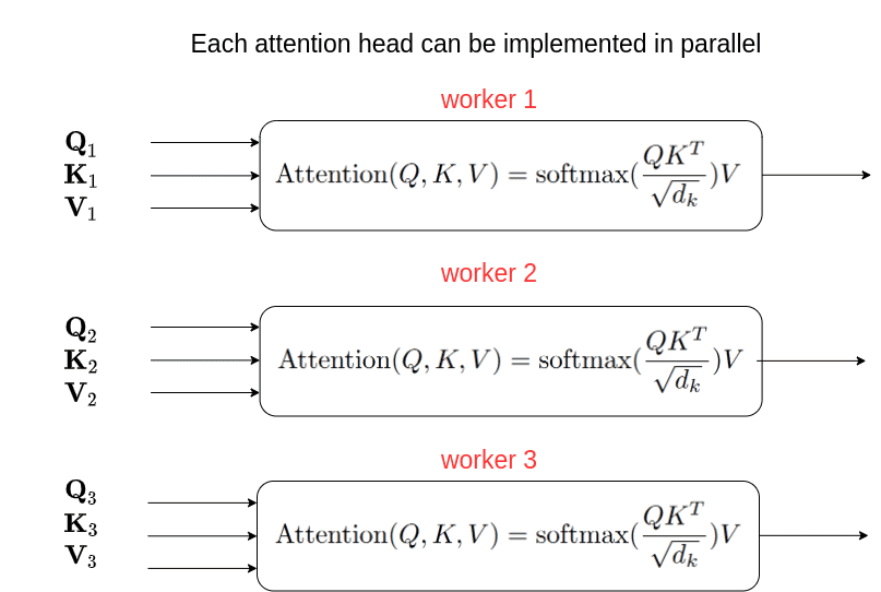
Interestingly, there are two types of parallel computations hidden inside self-attention:

by batching embedding vectors into the query matrix
by introducing multi-head attention.

We will analyze both. More importantly, I will try to provide different perspectives as to why multi-head self-attention works!

Please visit my introductory articles on attention and transformers for a high-level overview or our open-source lib for implementations.

Want to build your PyTorch fundamentals? Learn from the best ones on how to build Deep Learning models with PyTorch. Use the code aisummer35 to get an exclusive 35% discount from your favorite AI blog!

Self-attention as two matrix multiplications

The math

We will consider self dot-product attention without multiple heads to enhance readability. Given our inputs

\textbf{X} \in \mathcal{R}^{batch \times tokens \times d_{model}} ,

and trainable weight matrices:

\textbf{W}^{Q}, \textbf{W}^{K}, \textbf{W}^{V} \in \mathcal{R}^{d_{\text{model}} \times d_{k}}

$d_{model}$ is the size of the embedding vector of each input element from our sequence.
$d_k$ is the inner dimension of that is specific to each self-attention layer.
$batch$ is the batch size
$tokens$ is the number of elements that our sequence has.

We create 3 distinct representations ( the query, the key, and the value):

\textbf{Q} = \textbf{X} \textbf{W}^Q, \textbf{K} = \textbf{X} \textbf{W}^K, \textbf{V} = \textbf{X} \textbf{W}^V , \mathcal{R}^{batch \times tokens \times d_{k}}

Then, we can define the attention layer as:

\textbf{Y} = \operatorname{Attention}(\textbf{Q}, \textbf{K}, \textbf{V})=\operatorname{softmax}\left(\frac{\textbf{Q} \textbf{K}^{T}}{\sqrt{d_{k}}}\right) \textbf{V}

You might be wondering where is the attention weights. First, let's clarify that the attention is implemented as the dot-product and is happening right here:

\operatorname{Dot-scores} = \left(\frac{\textbf{Q} \textbf{K}^{T}}{\sqrt{d_{k}}}\right)

The higher the dot-product the higher the attention "weights" will be. That's why it is considered a similarity measure. Let’s see inside the math now.

An Intuitive illustration

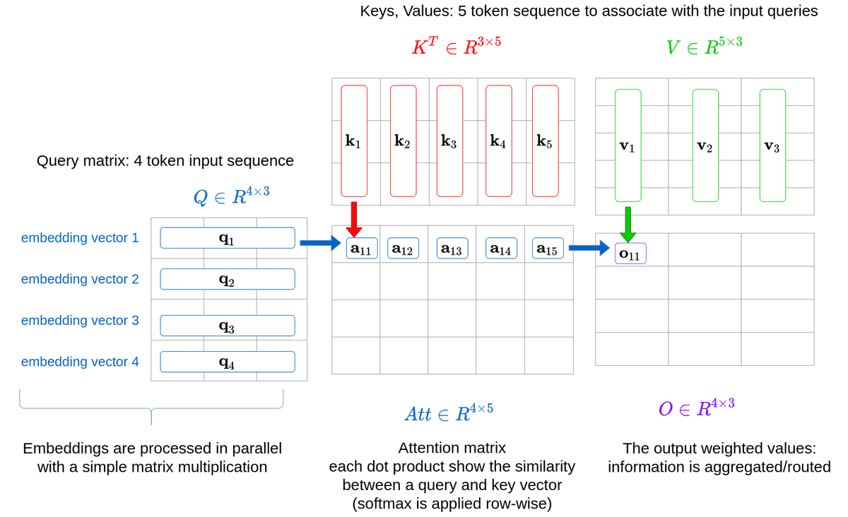
For the first illustration, we will consider a case wherein queries do not come from the same sequences as keys and vectors. Let’s say the query is a sequence of 4 tokens and the sequence that we would like to associate with, contains 5 tokens.

Both sequences contain vectors of the same embedding dimension, which is $d_model =3$ in our example. Then the self-attention can be defined as two matrix multiplications.

Take some time to analyze the following image:

Image by Author

By putting all the queries together, we have a matrix multiplication instead of a single query vector to matrix multiplication every time. Each query is processed completely independently from the others. This is the parallelization that we get for free by just using matrix multiplications and feeding all the input tokens/queries.

The Query-Key matrix multiplication

Content-based attention has distinct representations. The query matrix in the attention layer is conceptually the “search” in the database. The keys will account for where we will be looking while the values will actually give us the desired content. Consider the keys and values as components of our database.

Intuitively, the keys are the bridge between the queries (what we are looking for) and the values (what we will actually get).

Keep in mind that each vector to vector multiplication is a dot-product similarity. We can use the keys to guide our “search” and tell us where to look with respect to the input elements.

In other words, the keys will account for the computation of the attention on how to weigh the values based on our particular queries.

Notice that I did not show the softmax operation in the diagram, neither the scale-down factor $\sqrt{d_{k}}$ :

\alpha_{ij}=\frac{\exp \left(e_{i j}\right)}{\sum_{k=1}^{T_{x}} \exp \left(e_{i k}\right)}

The attention V matrix multiplication

Then the weights $\alpha_{ij}$ are used to get the final weighted value. For example, the outputs $o_{11},o_{12}, o_{13}$ will use the attention weights from the first query, as depicted in the diagram.

Cross attention of the vanilla transformer

The same principles apply in the encoder-decoder attention or alternatively cross attention, which makes complete sense:

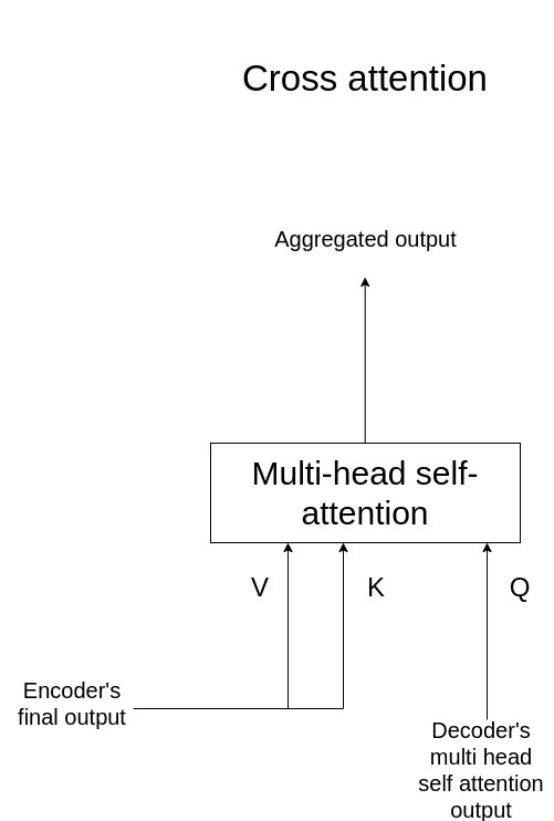Illustration of cross attention. Image by Author.

The keys and values are calculated by a linear projection of the final encoded input representation, after multiple encoder blocks.

How multi-head attention works in detail

Decomposing the attention in multiple heads is the second part of parallel and independent computations. Personally, I like to think of it as multiple “linear views” of the same sequence.

The original multi-head attention was defined as:

\text { MultiHead }(\textbf{Q}, \textbf{K}, \textbf{V}) =\text { Concat (head }_{1}, \ldots, \text { head } \left._{\mathrm{h}}\right) \textbf{W}^{O}

\text { where head }_{\mathrm{i}} =\text { Attention }\left(\textbf{Q} \textbf{W}_{i}^{Q}, \textbf{K} \textbf{W}_{i}^{K},\textbf{V} \textbf{W}_{i}^{V}\right)

Basically, the initial embedding dimension $dim$ is decomposed to $h \times d_{head}$ , and the computation per head is carried out independently.

See my article on implementing the self-attention mechanism for hands-on understanding on this subject.

The independent attention ‘heads’ are usually concatenated and multiplied by a linear layer to match the desired output dimension. The output dimension is often the same as the input embedding dimension $dim$ . This allows an easier stacking of multiple transformer blocks as well as identity skip connections.

I found an awesome illustration of the multiple heads from Peltarion’s blogpost:

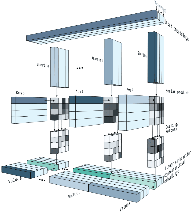Source: Getting meaning from text: self-attention step-by-step video, Peltarion blogpost

Intuitively, multiple heads enable us to attend independently to (parts of) the sequence.

If you like math and input-output diagrams, we got your back:

Image by Author

On the parallelization of independent computations of self-attention

Again, all the representations are created from the same input and merged together to produce a single output. However, the individual $Q_{i}, K_{i}, V_{i}$ are in a lower dimension $d_k = d_{model}/heads$ . The computations can be carried out independently as with the bach size. In fact, we make the same computation both for each batch and head.

Often, independent computations have a very easy parallelization process. Although, this depends on the underlying low-level implementation in the GPU threads. Ideally, we would assign a GPU thread for each batch and for each head. For instance, if we had batch=2 and heads=3 we can run the computations in 6 different threads. Since the dimension is $d_k = d_{model}/heads$ this would introduce, in theory, zero overhead. The overhead comes when concatenating the results and multiplying again with $W_{O}$ , which is minimal.

You probably were aware of the theory so far. Let’s delve into some interesting observations.

Insights and observations on the attention mechanism

Self-attention is not symmetric!

Because we tend to use the same input representation, don’t fall into the trap that self-attention is symmetric! I made this calamitous mistake when I started to understand transformers.

Insight 0: self-attention is not symmetric!

If you do the math it becomes trivial to understand:

\frac{\textbf{Q} \textbf{K}^{T}}{\sqrt{d_{k}}} = \frac{\textbf{X} \textbf{W}_Q (\textbf{X} \textbf{W}_K)^{T}}{\sqrt{d_{k}}} = \frac{\textbf{X} \textbf{W}_Q \textbf{W}_K^{T} \textbf{X}^T }{\sqrt{d_{k}}}

More specifically, if the Keys and Queries have the same amount of $N$ tokens, the attention matrix $N \times N$ can be interpreted as a directed graph:

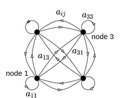A fully-connected graph with four vertices and sixteen directed bonds.Image from Gregory Berkolaiko. Source: ResearchGate

The arrows that correspond to weights can be regarded as a form of information routing.

In order for the self-attention to be symmetric, we would have to use the same projection matrix for the queries and the keys: $\textbf{W}_Q = \textbf{W}_K$ . That would make the presented graph undirected.

Why? Because when you multiply a matrix with its transpose you get a symmetric matrix. However, keep in mind that the rank of the resulted matrix will not be increased.

Inspired by this, there are many papers that use one shared projection matrix for the keys and the queries instead of two. More on that on multi-head attention.

Attention as the routing of multiple local information

Based on the ‘Enhancing the Transformer With Explicit Relational Encoding for Math Problem Solving’ paper:

Insight 1: “This (their results) indicates that the attention mechanism incorporates not just a subspace of the states it attends to, but affine transformations of those states that preserve nearly the full information content. In such a case, the attention mechanism can be interpreted as the routing of multiple local information sources into one global tree structure of local representations.” ~ Schlag et al.

We tend to think that multiple heads will allow the heads to attend to different parts of the input but this paper proves the initial guess wrong. The heads preserve almost all the content. This renders attention as a routing algorithm of the query sequence with respect to the key/values.

Encoder weights can be classified and pruned efficiently

In another work, Voita et al. [4] analyzed what happens when using multiple heads in their work “Analyzing Multi-Head Self-Attention: Specialized Heads Do the Heavy Lifting, the Rest Can Be Pruned”. They identified 3 types of important heads by looking at their attention matrices:

Positional heads that attend mostly to their neighbor.
Syntactic heads that point to tokens with a specific syntactic relation.
Heads that point to rare words in the sentence.

The best way to prove the significance of their head categorization is by pruning the others. Here is an example of their pruning strategy based on the head classification for the 48 heads (8 heads times 6 blocks) of the original transformer:

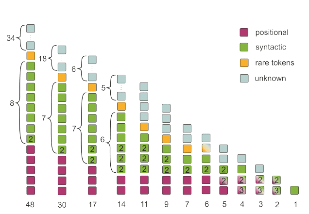Image by Voita et al. Source: Analyzing Multi-Head Self-Attention: Specialized Heads Do the Heavy Lifting, the Rest Can Be Pruned

By mostly keeping the heads that are classified in the distinguished categories, as shown, they managed to retain 17 out of 48 heads with almost the same BLEU score. Note that this corresponds to roughly 2⁄3 of the heads of the encoder.

Below are the results of pruning the Transformer’s encoder heads in two different datasets for machine translation:

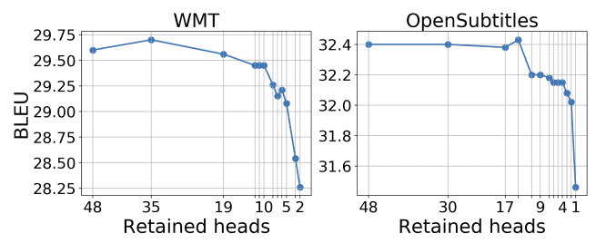Image by Voita et al. Source: Analyzing Multi-Head Self-Attention: Specialized Heads Do the Heavy Lifting, the Rest Can Be Pruned

Interestingly, the encoder attention heads were the easiest to prune, while encoder-decoder attention heads appear to be the most important for machine translation.

Insight 2: Based on the fact that the encoder-decoder attention heads are retained mostly in the last layers, it is highlighted that the first layers of the decoder account for language modeling, while the last layers for conditioning on the source sentence.

Another valuable paper in this direction is “Multi-Head Attention: Collaborate Instead of Concatenate” by Cordonnier et al.

The cumulative diagram depicts the sum of variances (in descending order for the X-axis) of the pretrained key and query matrices. The pretrained projection matrices are from a famous NLP model called BERT with $dim_{head}=64$ with 12 heads, which justifies $64 \cdot 12 = 768$ to study the matrix ranks.

The observation is based again on this equation:

\frac{\textbf{X} \textbf{W}_Q \textbf{W}_K^{T} \textbf{X}^T }{\sqrt{d_{k}}}

We will be looking into the pretrained projection product $\textbf{W}_K^{T} \textbf{X}^T$

Image by Cordonnier et al. Source: Multi-Head Attention: Collaborate Instead of Concatenate

The left figure depicts the product rank (in red) per head separately, while the right is per layer with concatenated heads.

Insight 3: Even though the separate product of the weight matrices per head is not low rank, the product of their concatenation (shown on the right, in red) is low rank.

This practically means that the heads share common projections. In other words, the phenomenally independent heads in fact learn to focus on the same subspaces.

Multiple heads on the encoder-decoder attention are super important

Paul Michel et al. [2] showed the importance of multiple heads when incrementally pruning heads from different attention submodels.

The following figure shows that performance drops much more rapidly when heads are pruned from the Encoder-Decoder attention layers (cross attention). The BLEU score is reported for machine translation.

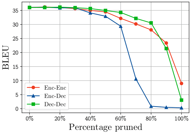Michel et al. Source: Are Sixteen Heads Really Better than One?

The authors show that pruning more than 60% of the cross attention heads of the vanilla transformer will result in significant performance degradation.

Insight 4: The encoder-decoder (cross) attention is significantly more dependent on the multi-headed decomposed representation.

After applying softmax, self-attention is low rank

Finally, there is a work by Sinong Wang et al. [7] that suggests that after applying softmax, self-attention of all the layers is of low rank.

P = \operatorname{softmax}\left(\frac{\textbf{Q} \textbf{K}^{T}}{\sqrt{d_{k}}}\right)

Again, the cumulative diagram depicts the sum of eigenvalues (in descending order for the X-axis). Broadly speaking, if the normalized cumulative sums up to 1 by using very few eigenvalues it means that these are the critical dimensions.

For the plot, they applied singular value decomposition into P across layers and heads of the pretrained model, and plot the normalized cumulative singular value averaged over 10k sentences

Source: Linformer: Self-Attention with Linear Complexity

Insight 5: After applying softmax, (self) attention is of low rank. This implies that a great part of the information contained in $P$ can be recovered from the first largest singular values (128 here).

Based on this observation, they proposed a simple linear attention mechanism by down-projecting the keys and values, called Linformer attention.

Attention weights as fast weight memory Systems

Context-dependent fast weight generation was introduced in the early 90s by Schmidhuber et al 1991. A slow net with slow weights continually generates fast weights for a fast net, making the fast weights effectively dependent on the context.

By removing the softmax in the well-known attention mechanism we have similar behavior.

\textbf{y}^{(i)} = \textbf{V}^{(i)} ( (\textbf{K}^{(i)})^T \textbf{q}^{(i)}) = (\textbf{V}^{(i)} (\textbf{K}^{(i)})^T)q^{(i)} = (\sum_{j=1}^i \textbf{v}^{(j)} \otimes \textbf{k}^{(j)} ) \textbf{q}^{(i)}

Where the outer product of values and keys can be regarded as the fast weights.

\textbf{W}^{(i)} = (\sum_{j=1}^i \textbf{v}^{(j)} \otimes \textbf{k}^{(i)} )

This is more or less the database, wherein:

\textbf{k}^{(i)}, \textbf{v}^{(i)}, \textbf{q}^{(i)} =\textbf{W}_k\textbf{x}^{(i)}, \textbf{W}_v\textbf{x}^{(i)}, \textbf{W}_q\textbf{x}^{(i)}

Finally, you get something that looks like the fast weights described in the 90’:

\textbf{y}^{(i)} = \textbf{W}^{(i)} \textbf{q}^{(i)}

Based on this observation, they discuss multiple ways to substitute the removal of the softmax operations and make associations to already proposed linear-complexity attention methods. Here is one insight that I liked from this work:

Insight 6: “As a consequence, to prevent associations from interfering with each other upon retrieval, the respective keys need to be orthogonal. Otherwise, the dot product will attend to more than one key and return a linear combination of values.” Schlag et al.

Yannic Kilcher analyzes this paper extensively in the following video:

Rank collapse and token uniformity

Recently, dong et al. [6] found that self-attention possesses an inductive bias towards token uniformity.

Insight 7: Surprising the audience, they noticed that without additional components such as MLP and skip-connections, the attention converges exponentially to a rank-1 matrix.

To this end, they studied mechanisms that are responsible to counteract rank collapse. In short, they found the following:

Skip connections are crucial: they prevent the transformer output from degenerating to rank one exponentially quickly with respect to network depth.
Multi-layer perceptrons that project the features in a higher dimension and the back to the initial dimension also help
Layer normalization plays no role in preventing rank collapse.

I’m betting that you might be wondering what Layer norm is useful for.

Layer norm: the key ingredient to transfer learning largely pretrained transformers

First of all, normalization methods are the key to stable training and faster convergence in the current dataset. However, their trainable parameters pose practical challenges for transfer learning.

In the transformer case, the paper “Pretrained Transformers As Universal Computation Engines” [10] provides some insights on fine-tuning only layer norm, which corresponds to the $\gamma$ and $\beta$ trainable parameters.

\mu_{n}=\frac{1}{K} \sum_{k=1}^{K} x_{nk}

\sigma_{n}^{2}=\frac{1}{K}\sum_{k=1}^{K}\left(x_{nk}-\mu_{n}\right)^{2}

\hat{x}_{nk}= \frac{x_{nk}-\mu_{n}}{\sqrt{\sigma_{n}^{2}+\epsilon}}, \hat{x}_{nk} \in R

\mathrm{LN}_{\gamma, \beta}\left(x_{n}\right) =\gamma \hat{x}_{n}+\beta ,x_{n} \in R^{K}

Intuitively, these parameters correspond to rescaling and shifting the attention signal.

They made huge ablation studies on the most critical components to be finetuned for datasets that belong to low-data regimes.

Insight 8: Surprisingly, the authors have found that the layer norm trainable parameters (0.1% of the parameters) to be the most crucial for fine-tuning transformers, after pretraining in huge (high data regime) natural language tasks [10].

You can imagine low-data regimes to domains where getting huge amounts of labeled data is costly and difficult like medical imaging. However, in their work, they use datasets such as MNIST and CIFAR-10 as low-data regime datasets. And they are compared to the huge amount of texts that a transformer can be pretrained on.

As it can be seen, the frozen transformer performs on par with the fully-fine-tuned transformer, which suggests two things:

Insight 9: Pretraning self-attention on massive natural language datasets results in excellent computational primitives.

Computation primitives are constructs or components which are not broken down (in a given context, such as a programming language or an atomic element of an expression in language). In other words, primitives are the smallest units of processing. And as it turns out, the learned Q, K, V projection matrices in these big NLP datasets learned transferable primitives.

Insight 10: Fine-tuning the attention layers can lead to performance divergence on small datasets.

On Quadratic Complexity: are we there yet?

We cannot conclude the attention mechanisms without indicating the huge amount of research spent on finding alternatives for their quadratic complexity. I will give you a short glimpse of what is happening in the following image from Yi Tay et al. 2020:

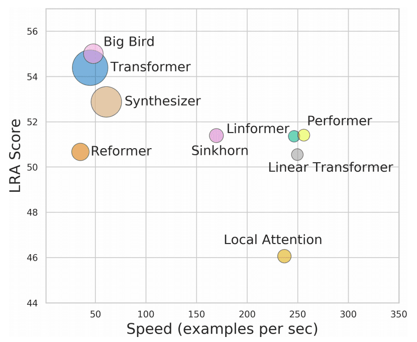Source: Long Range Arena: A Benchmark for Efficient Transformers

In general, there are two categories here:

Methods that use math to approximate the full quadratic global attention (all2all), like the Linformer that exploits matrix ranks.
Methods that try to constrict and sparsify attention. The most primitive example is “windowed” attention which is conceptually similar to convolutions (Figure (b) below). The most successful sparse-base method is Big Bird, as depicted below uses the combination of the above attention types.

Source: Big Bird: Transformers for Longer Sequences, by Zaheer et al.

Obviously, global attention is kept for the “special” tokens like the CLS token that is used for classification.

That being said, the path to reducing the quadratic complexity is far from over.

I am planning to provide a whole new article once the field becomes clear. Nonetheless, if you are serious about running some large sparse attention models check Deepspeed. It is one of the most famous and fast implementations of sparse transformers, developed by Microsoft. It provides GPU implementations for Pytorch with massive speedups.

Conclusion

After so many perspectives and observations, I hope you gained at least one new insight in the analysis of content-based attention. In my opinion, it is amazing how such a simple idea can have such immense impact and so many meanings and insights.

If you liked this article share it on social media so as to reach more curious people with similar questions. It would be highly appreciated, I give you my word!

Acknowledgment

A big shout out to Yannic Kilcher for explaining so many videos about transformers and attention. It is incredible that his videos accelerated the learning process of so many researchers around the globe.

References

[1] Vaswani, A., Shazeer, N., Parmar, N., Uszkoreit, J., Jones, L., Gomez, A. N., ... & Polosukhin, I. (2017). Attention is all you need. arXiv preprint arXiv:1706.03762.

[2] Michel, P., Levy, O., & Neubig, G. (2019). Are sixteen heads really better than one?. arXiv preprint arXiv:1905.10650.

[3] Cordonnier, J. B., Loukas, A., & Jaggi, M. (2020). Multi-Head Attention: Collaborate Instead of Concatenate. arXiv preprint arXiv:2006.16362.

[4] Voita, E., Talbot, D., Moiseev, F., Sennrich, R., & Titov, I. (2019). Analyzing multi-head self-attention: Specialized heads do the heavy lifting, the rest can be pruned. arXiv preprint arXiv:1905.09418.

[5] Schlag, I., Irie, K., & Schmidhuber, J. (2021). Linear Transformers Are Secretly Fast Weight Memory Systems. arXiv preprint arXiv:2102.11174.

[6] Yihe Dong et al. 2021. Attention is not all you need: pure attention loses rank doubly exponentially with depth

[7] Wang, S., Li, B., Khabsa, M., Fang, H., & Ma, H. (2020). Linformer: Self-attention with linear complexity. arXiv preprint arXiv:2006.04768.

[8] Tay, Y., Dehghani, M., Abnar, S., Shen, Y., Bahri, D., Pham, P., ... & Metzler, D. (2020). Long Range Arena: A Benchmark for Efficient Transformers. arXiv preprint arXiv:2011.04006.

[9] Zaheer, M., Guruganesh, G., Dubey, A., Ainslie, J., Alberti, C., Ontanon, S., ... & Ahmed, A. (2020). Big bird: Transformers for longer sequences. arXiv preprint arXiv:2007.14062.

[10] Lu, K., Grover, A., Abbeel, P., & Mordatch, I. (2021). Pretrained Transformers as Universal Computation Engines. arXiv preprint arXiv:2103.05247.

* Disclosure: Please note that some of the links above might be affiliate links, and at no additional cost to you, we will earn a commission if you decide to make a purchase after clicking through.

Why multi-head self attention works: math, intuitions and 10+1 hidden insights