How the Vision Transformer (ViT) works in 10 minutes: an image is worth 16x16 words

This time I am going to be sharp and short. In 10 minutes I will indicate the minor modifications of the transformer architecture for image classification.

Since it is a follow-up article feel free to advise my previous articles on Transformer and attention if you don’t feel that comfortable with the terms.

Now, ladies and gentlemen, you can start your clocks!

Transformers lack the inductive biases of Convolutional Neural Networks (CNNs), such as translation invariance and a locally restricted receptive field. You probably heard that before.

But what does it actually mean?

Well, invariance means that you can recognize an entity (i.e. object) in an image, even when its appearance or position varies. Translation in computer vision implies that each image pixel has been moved by a fixed amount in a particular direction.

Moreover, remember that convolution is a linear local operator. We see only the neighbor values as indicated by the kernel.

On the other hand, the transformer is by design permutation invariant. The bad news is that it cannot process grid-structured data. We need sequences! To this end, we will convert a spatial non-sequential signal to a sequence!

Let’s see how.

How the Vision Transformer works in a nutshell

The total architecture is called Vision Transformer (ViT in short). Let’s examine it step by step.

1. Split an image into patches

2. Flatten the patches

3. Produce lower-dimensional linear embeddings from the flattened patches

4. Add positional embeddings

5. Feed the sequence as an input to a standard transformer encoder

6. Pretrain the model with image labels (fully supervised on a huge dataset)

7. Finetune on the downstream dataset for image classification

Source: Google AI blog

Image patches are basically the sequence tokens (like words). In fact, the encoder block is identical to the original transformer proposed by Vaswani et al. (2017) as we have extensively described:

The well-know transformer block. Image by Alexey Dosovitskiy et al 2020. Source:An Image is Worth 16x16 Words: Transformers for Image Recognition at Scale

The only thing that changes is the number of those blocks. To this end, and to further prove that with more data they can train larger ViT variants, 3 models were proposed:

Alexey Dosovitskiy et al 2020. Source:An Image is Worth 16x16 Words: Transformers for Image Recognition at Scale

Heads refer to multi-head attention, while the MLP size refers to the blue module in the figure. MLP stands for multi-layer perceptron but it's actually a bunch of linear transformation layers.

Hidden size $D$ is the embedding size, which is kept fixed throughout the layers. Why keep it fixed? So that we can use short residual skip connections.

In case you missed it, there is no decoder in the game. Just an extra linear layer for the final classification called MLP head.

But is this enough?

Yes and no. Actually, we need a massive amount of data and as a result computational resources.

Important details

Specifically, if ViT is trained on datasets with more than 14M (at least :P) images it can approach or beat state-of-the-art CNNs.

If not, you better stick with ResNets or EfficientNets.

ViT is pretrained on the large dataset and then fine-tuned to small ones. The only modification is to discard the prediction head (MLP head) and attach a new $D \times K$ linear layer, where K is the number of classes of the small dataset.

I found it interesting that the authors claim that it is better to fine-tune at higher resolutions than pre-training.

To fine-tune in higher resolutions, 2D interpolation of the pre-trained position embeddings is performed. The reason is that they model positional embeddings with trainable linear layers. Having that said, the key engineering part of this paper is all about feeding an image in the transformer.

Representing an image as a sequence of patches

I was also super curious how you can elegantly reshape the image in patches. For an input image $\textbf(x) \in R^{H \times W \times C}$ and patch size $p$, we want to create $N$ image patches denoted as $\textbf(x)_p \in R^{N \times (P^{2} C)}$, where $N = \frac{H W}{P^{2}}$. $N$ is the sequence length similar to the words of a sentence.

If you didn’t notice the image patch i.e. [16,16,3] is flattened to 16x16x3. I hope by now the title makes sense ;)

I will use the einops library that works above PyTorch. You can install it via pip:

$ pip install einops

And then some compact Pytorch code:

from einops import rearrange

p = patch_size # P in maths

x_p = rearrange(img, 'b c (h p1) (w p2) -> b (h w) (p1 p2 c)', p1 = p, p2 = p)

In short, each symbol or each parenthesis indicates a dimension. For more information on einsum operations check out our blogpost on einsum operations.

Note that the image patches are always squares for simplicity.

And what about going from patch to embeddings? It’s just a linear transformation layer that takes a sequence of $P^{2} C$ elements and outputs $D$.

patch_dim = (patch_size**2) * channels # D in math

patch_to_embedding = nn.Linear(patch_dim, dim)

Can you see what’s missing?

I bet you do! We need to provide some sort of order.

Positional embeddings

Even though many positional embedding schemes were applied, no significant difference was found. This is probably due to the fact that the transformer encoder operates on a patch-level. Learning embeddings that capture the order relationships between patches (spatial information) is not so crucial. It is relatively easier to understand the relationships between patches of P x P than of a full image Height x Width.

Intuitively, you can imagine solving a puzzle of 100 pieces (patches) compared to 5000 pieces (pixels).

Hence, after the low-dimensional linear projection, a trainable position embedding is added to the patch representations. It is interesting to see what these position embeddings look like after training:

Alexey Dosovitskiy et al 2020. Source:An Image is Worth 16x16 Words: Transformers for Image Recognition at Scale

First, there is some kind of 2D structure. Second, patterns across rows (and columns) have similar representations. For high resolutions, a sinusoidal structure was used.

Key findings

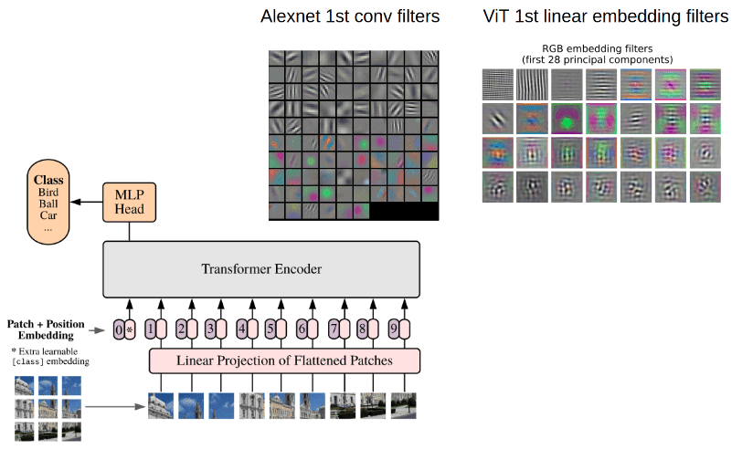
In the early conv days, we used to visualize the early layers.

Why?

Because we believe that well-trained networks often show nice and smooth filters.

Left: Alexnet fileters visualization. Source:Standford’s Course CS231n Right: ViT learned filters. Source:An Image is Worth 16x16 Words: Transformers for Image Recognition at Scale

I borrowed the image from Stanford's Course CS231n: Convolutional Neural Networks for Visual Recognition.

As it perfectly stated in CS231n:

“Notice that the first-layer weights are very nice and smooth, indicating a nicely converged network. The color/grayscale features are clustered because the AlexNet contains two separate streams of processing, and an apparent consequence of this architecture is that one stream develops high-frequency grayscale features and the other low-frequency color features.” ~ Stanford CS231 Course: Visualizing what ConvNets learn

For such visualizations PCA is used. In this way, the author showed that early layer representations may share similar features.

Next question please.

How far aways are the learned non-local interactions?

Short answer: For patch size P, maximum P*P, which in our case is 128, even from the 1st layer!

We don’t need successive conv. layers to get to 128-away pixels anymore. With convolutions without dilation, the receptive field is increased linearly. Using self-attention we have interaction between pixels representations in the 1st layer and pairs of representations in the 2nd layer and so on.

Right: Image generated using Fomoro AI calculator Left: Image by Alexey Dosovitskiy et al 2020

Based on the diagram on the left from ViT, one can argue that:

• There are indeed heads that attend to the whole patch already in the early layers.

• One can justify the performance gain based on the early access pixel interactions. It seems more critical for the early layers to have access to the whole patch (global info). In other words, the heads that belong to the upper left part of the image may be the core reason for superior performance.

• Interestingly, the attention distance increases with network depth similar to the receptive field of local operations.

• There are also attention heads with consistently small attention distances in the low layers. On the right, a 24-layer with standard 3x3 convolutions has a receptive field of less than 50. We would approximately need 50 conv layers, to attend to a ~100 receptive field, without dilation or pooling layers.

• To enforce this idea of highly localized attention heads, the authors experimented with hybrid models that apply a ResNet before the Transformer. They found less highly localized heads, as expected. Along with filter visualization, it suggests that it may serve a similar function as early convolutional layers in CNNs.

Attention distance and visualization

However, I find it critical to understand how they measured the mean attention distance. It’s analogous to the receptive field, but not exactly the same.

Attention distance was computed as the average distance between the query pixel and the rest of the patch, multiplied by the attention weight. They used 128 example images and averaged their results.

An example: if a pixel is 20 pixels away and the attention weight is 0.5 the distance is 10.

Finally, the model attends to image regions that are semantically relevant for classification, as illustrated below:

Alexey Dosovitskiy et al 2020. Source:An Image is Worth 16x16 Words: Transformers for Image Recognition at Scale

Implementation

Check out our repository to find self-attention modules for compute vision. Given an implementation of the vanilla Transformer Encoder, ViT looks as simple as this:

import torch
import torch.nn as nn
from einops import rearrange

from self_attention_cv import TransformerEncoder


class ViT(nn.Module):
    def __init__(self, *,
                 img_dim,
                 in_channels=3,
                 patch_dim=16,
                 num_classes=10,
                 dim=512,
                 blocks=6,
                 heads=4,
                 dim_linear_block=1024,
                 dim_head=None,
                 dropout=0, transformer=None, classification=True):
        """
        Args:
            img_dim: the spatial image size
            in_channels: number of img channels
            patch_dim: desired patch dim
            num_classes: classification task classes
            dim: the linear layer's dim to project the patches for MHSA
            blocks: number of transformer blocks
            heads: number of heads
            dim_linear_block: inner dim of the transformer linear block
            dim_head: dim head in case you want to define it. defaults to dim/heads
            dropout: for pos emb and transformer
            transformer: in case you want to provide another transformer implementation
            classification: creates an extra CLS token
        """
        super().__init__()
        assert img_dim % patch_dim == 0, f'patch size {patch_dim} not divisible'
        self.p = patch_dim
        self.classification = classification
        tokens = (img_dim // patch_dim) ** 2
        self.token_dim = in_channels * (patch_dim ** 2)
        self.dim = dim
        self.dim_head = (int(dim / heads)) if dim_head is None else dim_head
        self.project_patches = nn.Linear(self.token_dim, dim)

        self.emb_dropout = nn.Dropout(dropout)
        if self.classification:
            self.cls_token = nn.Parameter(torch.randn(1, 1, dim))
            self.pos_emb1D = nn.Parameter(torch.randn(tokens + 1, dim))
            self.mlp_head = nn.Linear(dim, num_classes)
        else:
            self.pos_emb1D = nn.Parameter(torch.randn(tokens, dim))

        if transformer is None:
            self.transformer = TransformerEncoder(dim, blocks=blocks, heads=heads,
                                                  dim_head=self.dim_head,
                                                  dim_linear_block=dim_linear_block,
                                                  dropout=dropout)
        else:
            self.transformer = transformer

    def expand_cls_to_batch(self, batch):
        """
        Args:
            batch: batch size
        Returns: cls token expanded to the batch size
        """
        return self.cls_token.expand([batch, -1, -1])

    def forward(self, img, mask=None):
        batch_size = img.shape[0]
        img_patches = rearrange(
            img, 'b c (patch_x x) (patch_y y) -> b (x y) (patch_x patch_y c)',
                                patch_x=self.p, patch_y=self.p)
        # project patches with linear layer + add pos emb
        img_patches = self.project_patches(img_patches)

        if self.classification:
            img_patches = torch.cat(
                (self.expand_cls_to_batch(batch_size), img_patches), dim=1)

        patch_embeddings = self.emb_dropout(img_patches + self.pos_emb1D)

        # feed patch_embeddings and output of transformer. shape: [batch, tokens, dim]
        y = self.transformer(patch_embeddings, mask)

        if self.classification:
            # we index only the cls token for classification. nlp tricks :P
            return self.mlp_head(y[:, 0, :])
        else:
            return y

Conclusion

The key engineering part of this work is the formulation of an image classification problem as a sequential problem by using image patches as tokens, and processing it by a Transformer. That sounds good and simple but it needs massive data. Unfortunately, Google owns the pretrained dataset so the results are not reproducible. And even if they were, you would need to have enough computing power.

Deep Learning in Production Book 📖

Learn how to build, train, deploy, scale and maintain deep learning models. Understand ML infrastructure and MLOps using hands-on examples.

Learn more

* Disclosure: Please note that some of the links above might be affiliate links, and at no additional cost to you, we will earn a commission if you decide to make a purchase after clicking through.