An overview of Unet architectures for semantic segmentation and biomedical image segmentation

A U-shaped architecture consists of a specific encoder-decoder scheme: The encoder reduces the spatial dimensions in every layer and increases the channels. On the other hand, the decoder increases the spatial dims while reducing the channels. The tensor that is passed in the decoder is usually called bottleneck. In the end, the spatial dims are restored to make a prediction for each pixel in the input image. These kinds of models are extremely utilized in real-world applications.

This article aims to explore the Unet architectures that stood the test of time.

To dive deeper into how AI is used in Medicine, you can't go wrong with this online course by Coursera: AI for Medicine

Fully Convolutional Network (FCN)

Fully convolutional network 1 was one of the first architectures without fully connected layers. Apart from the fact that it can be trained end-to-end, for individual pixel prediction (e.g semantic segmentation), it can process arbitrary-sized inputs. It is a general architecture that effectively uses transposed convolutions as a trainable upsampling method.

The fully convolutional layer architecture. Source

Given a pretrained encoder here is what an FCN looks like:

import torch
import torch.nn as nn

class FCN32s(nn.Module):

    def __init__(self, pretrained_net, n_class):
        super().__init__()
        self.n_class = n_class
        self.pretrained_net = pretrained_net
        self.relu   = nn.ReLU(inplace=True)
        self.deconv1 = nn.ConvTranspose2d(512, 512, kernel_size=3, stride=2, padding=1, dilation=1, output_padding=1)
        self.bn1    = nn.BatchNorm2d(512)
        self.deconv2 = nn.ConvTranspose2d(512, 256, kernel_size=3, stride=2, padding=1, dilation=1, output_padding=1)
        self.bn2    = nn.BatchNorm2d(256)
        self.deconv3 = nn.ConvTranspose2d(256, 128, kernel_size=3, stride=2, padding=1, dilation=1, output_padding=1)
        self.bn3    = nn.BatchNorm2d(128)
        self.deconv4 = nn.ConvTranspose2d(128, 64, kernel_size=3, stride=2, padding=1, dilation=1, output_padding=1)
        self.bn4    = nn.BatchNorm2d(64)
        self.deconv5 = nn.ConvTranspose2d(64, 32, kernel_size=3, stride=2, padding=1, dilation=1, output_padding=1)
        self.bn5    = nn.BatchNorm2d(32)
        self.classifier = nn.Conv2d(32, n_class, kernel_size=1)

    def forward(self, x):
        output = self.pretrained_net(x)
        x5 = output['x5']  # size=(N, 512, x.H/32, x.W/32)

        score = self.bn1(self.relu(self.deconv1(x5)))   # size=(N, 512, x.H/16, x.W/16)
        score = self.bn2(self.relu(self.deconv2(score)))  # size=(N, 256, x.H/8, x.W/8)
        score = self.bn3(self.relu(self.deconv3(score)))  # size=(N, 128, x.H/4, x.W/4)
        score = self.bn4(self.relu(self.deconv4(score)))  # size=(N, 64, x.H/2, x.W/2)
        score = self.bn5(self.relu(self.deconv5(score)))  # size=(N, 32, x.H, x.W)
        score = self.classifier(score)                  # size=(N, n_class, x.H/1, x.W/1)

        return score

You can even load a pretrained model from pytorch hub:

import torch
model = torch.hub.load('pytorch/vision:v0.9.0', 'fcn_resnet101', pretrained=True)
model.eval()

Note that all pre-trained models expect input images normalized in the same way, i.e. mini-batches of 3-channel RGB images of shape (N, 3, H, W), where N is the number of images, H and W are expected to be at least 224 pixels. The images have to be loaded in to a range of [0, 1] and then normalized using mean = [0.485, 0.456, 0.406] and std = [0.229, 0.224, 0.225]

U-Net and 3D U-Net

Later on, Unet modifies and extends FCN.

The main idea is to make FCN maintain the high-level features in the early layer of the decoder. To this end, they introduce long skip-connections to localize the segmentations.

In this manner, high-resolution features (but semantically low) from the encoder path are combined and reused with the upsampled output. Unet is also a symmetric architecture, as depicted below.

The Unet model. Source

It can be divided into an encoder-decoder path or contracting-expansive path equivalently.

Encoder (left side): It consists of the repeated application of two 3x3 convolutions. Each conv is followed by a ReLU and batch normalization. Then a 2x2 max pooling operation is applied to reduce the spatial dimensions. Again, at each downsampling step, we double the number of feature channels, while we cut in half the spatial dimensions.

Decoder path (right side): Every step in the expansive path consists of an upsampling of the feature map followed by a 2x2 transpose convolution, which halves the number of feature channels. We also have a concatenation with the corresponding feature map from the contracting path, and usually a 3x3 convolutional (each followed by a ReLU). At the final layer, a 1x1 convolution is used to map the channels to the desired number of classes.

Here is an implementation of 2D Unet

import torch
import torch.nn as nn
import torch.nn.functional as F


class DoubleConv(nn.Module):
    def __init__(self, in_ch, out_ch):
        super(DoubleConv, self).__init__()
        self.conv = nn.Sequential(
            nn.Conv2d(in_ch, out_ch, 3, padding=1),
            nn.BatchNorm2d(out_ch),
            nn.ReLU(inplace=True),
            nn.Conv2d(out_ch, out_ch, 3, padding=1),
            nn.BatchNorm2d(out_ch),
            nn.ReLU(inplace=True))

    def forward(self, x):
        x = self.conv(x)
        return x


class InConv(nn.Module):
    def __init__(self, in_ch, out_ch):
        super(InConv, self).__init__()
        self.conv = DoubleConv(in_ch, out_ch)

    def forward(self, x):
        x = self.conv(x)
        return x


class Down(nn.Module):
    def __init__(self, in_ch, out_ch):
        super(Down, self).__init__()
        self.mpconv = nn.Sequential(
            nn.MaxPool2d(2),
            DoubleConv(in_ch, out_ch)
        )

    def forward(self, x):
        x = self.mpconv(x)
        return x


class Up(nn.Module):
    def __init__(self, in_ch, out_ch, bilinear=True):
        super(Up, self).__init__()

        if bilinear:
            self.up = nn.Upsample(scale_factor=2, mode='bilinear', align_corners=True)
        else:
            self.up = nn.ConvTranspose2d(in_ch // 2, in_ch // 2, 2, stride=2)

        self.conv = DoubleConv(in_ch, out_ch)

    def forward(self, x1, x2):
        x1 = self.up(x1)

        diffY = x2.size()[2] - x1.size()[2]
        diffX = x2.size()[3] - x1.size()[3]

        x1 = F.pad(x1, (diffX // 2, diffX - diffX // 2,
                        diffY // 2, diffY - diffY // 2))
        x = torch.cat([x2, x1], dim=1)
        x = self.conv(x)
        return x


class OutConv(nn.Module):
    def __init__(self, in_ch, out_ch):
        super(OutConv, self).__init__()
        self.conv = nn.Conv2d(in_ch, out_ch, 1)

    def forward(self, x):
        x = self.conv(x)
        return x

class Unet(nn.Module):
    def __init__(self, in_channels, classes):
        super(Unet, self).__init__()
        self.n_channels = in_channels
        self.n_classes =  classes

        self.inc = InConv(in_channels, 64)
        self.down1 = Down(64, 128)
        self.down2 = Down(128, 256)
        self.down3 = Down(256, 512)
        self.down4 = Down(512, 512)
        self.up1 = Up(1024, 256)
        self.up2 = Up(512, 128)
        self.up3 = Up(256, 64)
        self.up4 = Up(128, 64)
        self.outc = OutConv(64, classes)

    def forward(self, x):
        x1 = self.inc(x)
        x2 = self.down1(x1)
        x3 = self.down2(x2)
        x4 = self.down3(x3)
        x5 = self.down4(x4)
        x = self.up1(x5, x4)
        x = self.up2(x, x3)
        x = self.up3(x, x2)
        x = self.up4(x, x1)
        x = self.outc(x)
        return x

This method has great success in 2D biomedical image segmentation. And it is still used as a baseline method. But what about 3D images?

The 3D-Unet

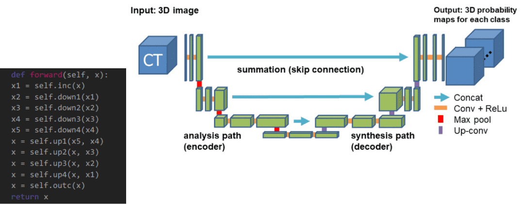
3D Unet was introduced shortly after Unet to process volumes. Only 3 layers are shown in the official diagram but in practice, we use more when we implement this model. Each block uses batch normalization after the convolution.

The 3D Unet model. Source

V-Net (2016)

Vnet extends Unet to process 3D MRI volumes. In contrast to processing the input 3D volumes slice-wise, they proposed to use 3D convolutions. In the end, medical images have an inherent 3D structure, and slice-wise processing is sub-optimal. The main modifications of Vnet are:

Motivated by similar works on image classification, they replaced max-pooling operations with strided convolutions. This is performed through convolution with 2 × 2 × 2 kernels applied with stride 2.
3D convolutions with padding are performed in each stage using 5×5×5 kernels.
Short residual connections are also employed in both parts of the network.
They use 3D transpose convolutions in order to increase the size of the inputs, followed by one to three conv layers. Feature maps are halved in every decoder layer.

All the above can be illustrated in this image:

The Vnet model. Source

Finally, in this work, the Dice loss was introduced which is a common loss function in segmentation. You can find the implementation of Vnet in our open-source library.

UNet++ (2018)

Motivation: The skip connections used in U-Net directly fast-forward high-resolution feature maps from the encoder to the decoder network. This results in the concatenation of semantically dissimilar feature maps.

The main idea behind UNet++ is to bridge the semantic gap between the feature maps of the encoder and decoder before concatenation. To this end, UNet++ is based on both nested and dense skip connections. UNet++ can effectively capture fine-grained details of 2D images. Visually:

UNet++ consists of an encoder and decoder that are connected through a series of nested dense convolutional blocks. Image by Unet++ paper. Source

In the above image, black indicates the original U-Net, while green and blue show dense convolution blocks on the skip pathways. Red indicates deep supervision, meaning there are multiple loss terms, as opposed to standard Unet. The implementation is publicly available.

In other words, the dense convolution block brings the semantic level of the encoder feature maps closer to that of the feature maps awaiting in the decoder. However, the number of parameters as well as the time to train the network is significantly higher. This is the main reason that there is no similar architecture with 3D convolutions.

No New-Net (2018)

The established Unet baseline for semantic image segmentation. It was tested on the BRATS dataset with top ranked results. Main points:

It uses 128x128x128 sub-volumes with a batch size of two
30 channels in the first conv layer
Trilinear upsampling in the decoder
Combine Dice loss with negative log-likelihood
Augmentation strategy: random rotations, random scaling, random elastic deformations, gamma correction augmentation and mirroring.
A l2 weight decay of $10^{−5}$

Image by Fabian Isensee et al. Source

A detailed walk-through Github repo is available.

MRI brain tumor segmentation in 3D using autoencoder regularization

Even though this is not exactly a conventional Unet architecture it deserves to belong in the list. The encoder is a 3D Resenet model and the decoder uses transpose convolutions. The first crucial part is the green building block, as illustrated in the diagram:

Image by Andriy Myronenko et al. Source

It uses successive padded 3D convolutions with group normalization, relu activations, and residual skip connections.

The second import component is the subnetwork on the bottom right: it is a Variational autoencoder that tries to reconstruct the original 3D input image.

Why?

Good question!

The motivation for using the auto-encoder branch is to provide extra guidance and regularization to the encoder part, since the training data are limited.

Even though this model uses a huge amount of GPU memory it won the BRATS competition. Implementation is publicly available in the MedicalZoo library.

MultiResUNet : Rethinking the U-Net Architecture for Multimodal Biomedical Image Segmentation (2020)

Medical images originate from various modalities and the segmentations we care about are of irregular and different scales. To address this, they proposed to use inception-like conv modules. Here is a quick recap of how the Inception module works:

Following the Inception network, they augment U-Net with multi-resolutions by incorporating 3 x 3, and 7 x 7 convolution operations in parallel to the existing 3x3 conv.

An inception-like block to capture multiple scales. Image by Nabil Ibtehaz et al. Source

To deal with the additional network complexity, they factorize the 5 x 5 and 7 x 7 convolutional layers, using a sequence of small 3 x 3 convolutional blocks. Then the outputs from the three convolutional blocks are concatenated to extract the spatial features from different scales.

Additionally, they gradually increase the filters in the succeeding conv, to reduce the memory footprint of the earlier layers. Finally, they add a short residual skip connection and introduce a pointwise (1 x 1) conv layer, which may assist us to capture additional spatial information.

Image by Nabil Ibtehaz et al. Source

To tackle the divergence between the encoder-decoder features (due to long skip connections), they propose to incorporate some convolutional layers along the shortcut connections. The hypothesis is that the additional non-linear transformations should compensate the further processing done during the decoder stage.

Alternating skip connections. Image by Nabil Ibtehaz et al. Source

These architectural inception-like improvements demonstrated superior results in many medical image segmentation datasets. Try it yourself to find out more.

The 3D U^2-Net: introducing channel-wise separable convolutions

Depth-wise means that the computation is performed across the different channels (channel-wise).

In separable convolution, the computation is factorized into two sequential steps: a channel-wise that processes channels independently and another 1x1xchannel conv that merges the independently produced feature maps.

Again, channel-wise convolution applies an independent convolutional filter per input channel,as depicted:

Image by Chi-Feng Wang. Source

The pointwise (1x1xk or 1x1x1xk kernel) convolution combines linearly the

output across all channels for every spatial location.

Image by Chi-Feng Wang. Source

For the 3D case the parameter gain is enormous, especially when training multiple instances of the model on different domains, denoted by $T$ . A 3x3x3 conv layer with input channels $c_{in}$ and out channels $c_{out}$ need $27 ∗ c_{in} ∗ c_{out} ∗ T$ parameters. With separable convolutions the total number of weights in the above filter is $(27 ∗ c_{in} ∗ T) + (c_{in} ∗ c_{out})$ .

The main assumption is that each domain has its own channel-wise filters, while pointwise conv kernels are shared.

Image by Chao Huang et al. Source

The input layer uses 16 filters. The encoder and decoder paths both contain five levels at different resolutions. Residual skip connection is applied within each level. Skip connection is employed to preserve more contextual information from the encoder counterpart for decoder path.

Obviously, the proposed 3D $U^2$ -Net requires the least parameters, indicating that it can perform effectively across various domains. The overall number of parameters from the universal model is around 1% of that of all independent models, while the two obtain comparable segmentation accuracy. Code is also publicly available.

Conclusion

To conclude, there is no one size fits all model. I tried to provide a general set of experimentally validated ideas to work around Unet. Feel free to try some of them out. There is this git repo that collects Unet architectures with links to code. Last but not least, feedback is always welcome! Let me know what you think on our social pages.

To dive deeper into how AI is used in Medicine, we highly recommend the Coursera course AI for Medicine

References

[1] Long, J., Shelhamer, E., & Darrell, T. (2015). Fully convolutional networks for semantic segmentation. In Proceedings of the IEEE conference on computer vision and pattern recognition (pp. 3431-3440).
[2] Ronneberger, O., Fischer, P., & Brox, T. (2015, October). U-net: Convolutional networks for biomedical image segmentation. In International Conference on Medical image computing and computer-assisted intervention (pp. 234-241). Springer, Cham.
[3] Milletari, F., Navab, N., & Ahmadi, S. A. (2016, October). V-net: Fully convolutional neural networks for volumetric medical image segmentation. In 2016 fourth international conference on 3D vision (3DV) (pp. 565-571). IEEE.
[4] Çiçek, Ö., Abdulkadir, A., Lienkamp, S. S., Brox, T., & Ronneberger, O. (2016, October). 3D U-Net: learning dense volumetric segmentation from sparse annotation. In International conference on medical image computing and computer-assisted intervention (pp. 424-432). Springer, Cham.
[5] Zhou, Z., Siddiquee, M. M. R., Tajbakhsh, N., & Liang, J. (2018). Unet++: A nested u-net architecture for medical image segmentation. In Deep Learning in Medical Image Analysis and Multimodal Learning for Clinical Decision Support (pp. 3-11). Springer, Cham.
[6] Wang, W., Yu, K., Hugonot, J., Fua, P., & Salzmann, M. (2019). Recurrent U-Net for resource-constrained segmentation. In Proceedings of the IEEE International Conference on Computer Vision (pp. 2142-2151).
[7] Huang, C., Han, H., Yao, Q., Zhu, S., & Zhou, S. K. (2019, October). 3D U^2-Net: A 3D Universal U-Net for Multi-domain Medical Image Segmentation. In International Conference on Medical Image Computing and Computer-Assisted Intervention (pp. 291-299). Springer, Cham.
[8] Ibtehaz, N., & Rahman, M. S. (2020). MultiResUNet: Rethinking the U-Net architecture for multimodal biomedical image segmentation. Neural Networks, 121, 74-87.
[9] Isensee, F., Kickingereder, P., Wick, W., Bendszus, M., & Maier-Hein, K. H. (2018, September). No new-net. In International MICCAI Brainlesion Workshop (pp. 234-244). Springer, Cham.
[10] Oktay, O., Schlemper, J., Folgoc, L. L., Lee, M., Heinrich, M., Misawa, K., ... & Glocker, B. (2018). Attention u-net: Learning where to look for the pancreas. arXiv preprint arXiv:1804.03999.
[11] Alom, M. Z., Hasan, M., Yakopcic, C., Taha, T. M., & Asari, V. K. (2018). Recurrent residual convolutional neural network based on u-net (r2u-net) for medical image segmentation. arXiv preprint arXiv:1802.06955.
[12] Myronenko, A. (2018, September). 3D MRI brain tumor segmentation using autoencoder regularization. In International MICCAI Brainlesion Workshop (pp. 311-320). Springer, Cham.

* Disclosure: Please note that some of the links above might be affiliate links, and at no additional cost to you, we will earn a commission if you decide to make a purchase after clicking through.