When I realized that I cannot apply common image processing pipelines in medical images, I was completely discouraged. Why does such functionality not exist? So, I made up this post (plus a notebook) for discouraged individuals who, like me, are interested in solving medical imaging problems.
We have already discussed medical image segmentation and some initial background on coordinate systems and DICOM files. My experience in the field leads me to continue with data understanding, preprocessing, and some augmentations. As I always say, if you merely understand your data and their particularities, you are probably playing bingo. In the field of medical imaging, I find some data manipulations, which are heavily used in preprocessing and augmentation in state-of-the-art methods, to be critical in our understanding. To this end, I provide a notebook for everyone to play around. It performs transformations on medical images, which is simply a 3D structured grid.
To dive deeper into how AI is used in Medicine, you can’t go wrong with the AI for Medicine online course, offered by Coursera. If you want to focus on medical image analysis with deep learning, I highly recommend starting from the Pytorch-based Udemy Course.
Data: We will play with 2 MRI images that are provided from nibabel (python library) for illustration purposes. The images are stored as nifty files. But before that, let’s write up some code to visualize the 3D medical volumes.
The images will be shown in 3 planes: sagittal, coronal, axial looking from left to right throughout this post.
Two-dimensional planes visualization
Throughout the whole tutorial, we will extensively use a function that visualizes the three median slices in the sagittal, coronal, and axial planes respectively. Let’s write some minimal function to do so:
def show_mid_slice(img_numpy, title='img'):"""Accepts an 3D numpy array and shows median slices in all three planes"""assert img_numpy.ndim == 3n_i, n_j, n_k = img_numpy.shape# sagittal (left image)center_i1 = int((n_i - 1) / 2)# coronal (center image)center_j1 = int((n_j - 1) / 2)# axial slice (right image)center_k1 = int((n_k - 1) / 2)show_slices([img_numpy[center_i1, :, :],img_numpy[:, center_j1, :],img_numpy[:, :, center_k1]])plt.suptitle(title)def show_slices(slices):"""Function to display a row of image slicesInput is a list of numpy 2D image slices"""fig, axes = plt.subplots(1, len(slices))for i, slice in enumerate(slices):axes[i].imshow(slice.T, cmap="gray", origin="lower")
Nothing more than matplotlib’s “imshow" and numpy’s array manipulations. For the record, medical images are a single channel and we visualize them in grayscale colors.
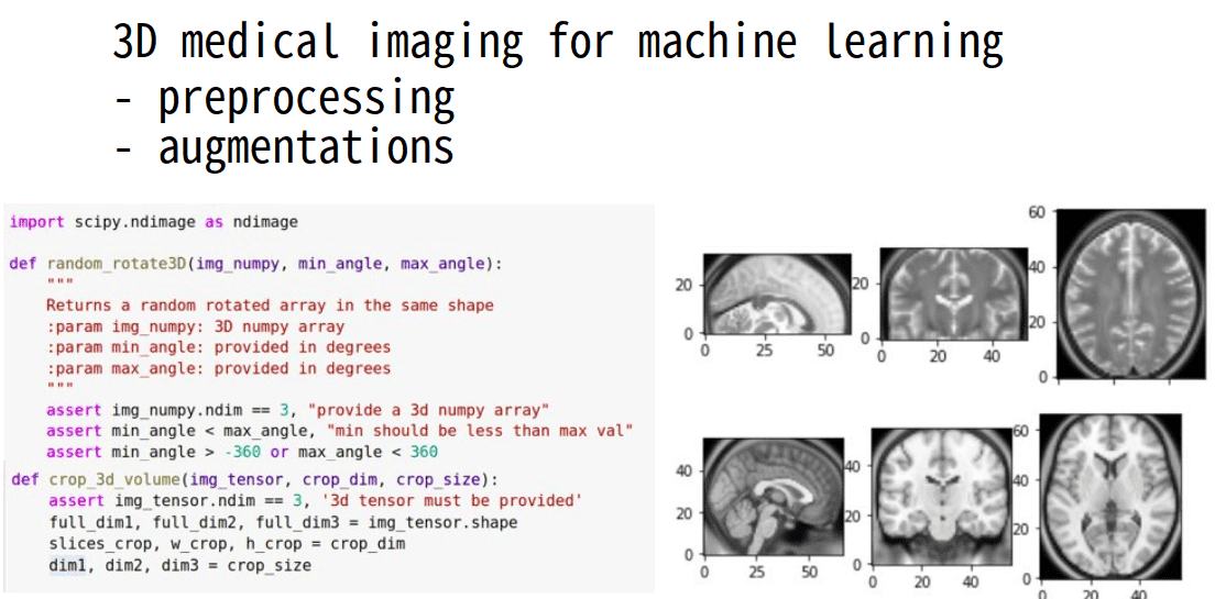
The two images that we will use to play with a plethora of transformations can be illustrated below:
show_mid_slice(epi_img_numpy, 'first image')show_mid_slice(anatomy_img_numpy,'second image')
 The initial brain MRI images that we will use.
Now we are good to go! Let’s commence with resize and rescale in medical images. Yeap, it’s not exactly the same.
Medical image resizing (down/up-sampling)
The scipy library provides a lot of functionalities for multi-dimensional images. Since medical images are three dimensional, a lot of functionalities can be used. This time we will use scipy.ndimage.interpolation.zoom for resizing the image in the desired dimensions. This is similar to downsampling in a 2D image. The same function can be used for interpolation to increase the spatial dimensions. As an illustration, we will double and half the original image size.
Keep in mind that in this kind of transformation the ratios are usually important to be maintained.
You probably don’t want to lose the anatomy of the human body :)
import scipydef resize_data_volume_by_scale(data, scale):"""Resize the data based on the provided scale"""scale_list = [scale,scale,scale]return scipy.ndimage.interpolation.zoom(data, scale_list, order=0)result = resize_data_volume_by_scale(epi_img_numpy, 0.5)result2 = resize_data_volume_by_scale(epi_img_numpy, 2)
This kind of scaling is usually called isometric. Honestly, I am not a big fan of the scipy's terminology to use the word zoom for this functionality.
 Downsampled and upsampled image by a factor of 2
It is very common to downsample the image in a lower dimension for heavy machine learning.
Note that there is another type of resizing. Instead of providing the desired output shape, you specify the desired voxel size(i.e. voxel_size=(1,1,1) mm). Nibabel provides a function called resample_to_output(). It works with nifti files and not with numpy arrays. Honestly, I wouldn't recommend it alone since the resulting images might not have the same shape. This may be a problem for deep learning. For example to create batches with dataloaders the dimension should be consistent across instances. However, you may choose to include it in a previous step in your pipeline. It can be used to bring different images to have the same or similar voxel size.
Medical image rescaling (zoom- in/out)
Rescaling can be regarded as an affine transformation. We will randomly zoom in and out of the image. This augmentation usually helps the model to learn scale-invariant features.
def random_zoom(matrix,min_percentage=0.7, max_percentage=1.2):z = np.random.sample() *(max_percentage-min_percentage) + min_percentagezoom_matrix = np.array([[z, 0, 0, 0],[0, z, 0, 0],[0, 0, z, 0],[0, 0, 0, 1]])return ndimage.interpolation.affine_transform(matrix, zoom_matrix)
 Random zoom in and zoom out
It is important to see that the empty area is filled with black pixels (zero intensity).
Note here that the surrounding air in medical images does not have zero intensity. Black is really relative to medical images.
The next one on the list is 3D rotation.
Medical image rotation
Rotation is one of the most common methods to achieve data augmentation in computer vision. It has also been considered a self-supervised technique with remarkable results [Spyros Gidaris et al. ].
In medical imaging, it is an equal import functionality that has also been used from self-supervised pretraining [Xinrui Zhuang et al. 2019 ]. A simple random 3D rotation in a given range of degrees can be illustrated with the code below:
def random_rotate3D(img_numpy, min_angle, max_angle):"""Returns a random rotated array in the same shape:param img_numpy: 3D numpy array:param min_angle: in degrees:param max_angle: in degrees"""assert img_numpy.ndim == 3, "provide a 3d numpy array"assert min_angle < max_angle, "min should be less than max val"assert min_angle > -360 or max_angle < 360all_axes = [(1, 0), (1, 2), (0, 2)]angle = np.random.randint(low=min_angle, high=max_angle+1)axes_random_id = np.random.randint(low=0, high=len(all_axes))axes = all_axes[axes_random_id]return scipy.ndimage.rotate(img_numpy, angle, axes=axes)
 Random 3D rotation
We simply have to define the axis and the rotation angle. As scaling provided the model with more diversity in order to learn scale-invariant features, rotation aids in learning rotation-invariant features.
Next in our list is image flipping.
Medical image flip
Similar to common RGB images, we can perform axis flipping in medical images. At this point, it is really important to clarify one thing:
When we perform augmentations and/or preprocessing in our data, we may have to apply similar operations on the ground truth data.
For instance, if we tackle the task of medical image segmentation, it is important to flip the target segmentation map. A simple implementation can be found below:
def random_flip(img, label=None):axes = [0, 1, 2]rand = np.random.randint(0, 3)img = flip_axis(img, axes[rand])img = np.squeeze(img)if label is None:return imgelse:y = flip_axis(y, axes[rand])y = np.squeeze(y)return x, ydef flip_axis(x, axis):x = np.asarray(x).swapaxes(axis, 0)x = x[::-1, ...]x = x.swapaxes(0, axis)return x
 The initial image as a reference and two flipped versions
Observe that by flipping one axis, two views change. The first image on top is the initial image as a reference.
Medical image shifting (displacement)
Here I would like to tell something else.
Rotation, shifting, and scaling are nothing more than affine transformations.
Sometimes I implement them by just defining the affine transformations and apply it in the image with scipy, and sometimes I use the already-implemented functions for multi-dimensional image processing.
In order to use this operation in my data augmentation pipeline, you can see that I have included a wrapper function. The latter basically samples a random number, usually in the desired range, and calls the affine transformation function. Below is the implementation for random shifting/displacement.
def transform_matrix_offset_center_3d(matrix, x, y, z):offset_matrix = np.array([[1, 0, 0, x], [0, 1, 0, y], [0, 0, 1, z], [0, 0, 0, 1]])return ndimage.interpolation.affine_transform(matrix, offset_matrix)def random_shift(img_numpy, max_percentage=0.4):dim1, dim2, dim3 = img_numpy.shapem1,m2,m3 = int(dim1*max_percentage/2),int(dim1*max_percentage/2), int(dim1*max_percentage/2)d1 = np.random.randint(-m1,m1)d2 = np.random.randint(-m2,m2)d3 = np.random.randint(-m3,m3)return transform_matrix_offset_center_3d(img_numpy, d1, d2, d3)
 The displaced medical images
This augmentation is not very common in medical image augmentation, but we include them here for completeness.
The reason we do not include it is that convolutional neural networks are by definition designed to learn translation-invariant features.
Random 3D crop
Cropping is not significantly different from natural images also. However, keep in mind that we usually have to take all the slices of a dimension and we need to take care of that. The reason is that one dimension may have fewer slices than the others. For example, one time I had to deal with a 384x384x64 image, which is common in CT images.
def crop_3d_volume(img_tensor, crop_dim, crop_size):assert img_tensor.ndim == 3, '3d tensor must be provided'full_dim1, full_dim2, full_dim3 = img_tensor.shapeslices_crop, w_crop, h_crop = crop_dimdim1, dim2, dim3 = crop_size# check if crop size matches image dimensionsif full_dim1 == dim1:img_tensor = img_tensor[:, w_crop:w_crop + dim2,h_crop:h_crop + dim3]elif full_dim2 == dim2:img_tensor = img_tensor[slices_crop:slices_crop + dim1, :,h_crop:h_crop + dim3]elif full_dim3 == dim3:img_tensor = img_tensor[slices_crop:slices_crop + dim1, w_crop:w_crop + dim2, :]# standard cropelse:img_tensor = img_tensor[slices_crop:slices_crop + dim1, w_crop:w_crop + dim2,h_crop:h_crop + dim3]return img_tensordef find_random_crop_dim(full_vol_dim, crop_size):assert full_vol_dim[0] >= crop_size[0], "crop size is too big"assert full_vol_dim[1] >= crop_size[1], "crop size is too big"assert full_vol_dim[2] >= crop_size[2], "crop size is too big"if full_vol_dim[0] == crop_size[0]:slices = crop_size[0]else:slices = np.random.randint(full_vol_dim[0] - crop_size[0])if full_vol_dim[1] == crop_size[1]:w_crop = crop_size[1]else:w_crop = np.random.randint(full_vol_dim[1] - crop_size[1])if full_vol_dim[2] == crop_size[2]:h_crop = crop_size[2]else:h_crop = np.random.randint(full_vol_dim[2] - crop_size[2])return (slices, w_crop, h_crop)
 Random cropping example
There are other techniques for cropping that focus on the area that we are interested i.e. the tumor, but we will not get into that now.
So far we played with geometrical transformations. Let’s see what we can do with the intensity of the image.
Clip intensity values (outliers)
This step is not applicable for this tutorial, but it may come in quite useful in general. Especially for CT images. The reason it is not applicable is that the MRI images are in a pretty narrow range of values.
def percentile_clip(img_numpy, min_val=5, max_val=95):"""Intensity normalization based on percentileClips the range based on the quartile values.:param min_val: should be in the range [0,100]:param max_val: should be in the range [0,100]:return: intensity normalized image"""low = np.percentile(img_numpy, min_val)high = np.percentile(img_numpy, max_val)img_numpy[img_numpy < low] = lowimg_numpy[img_numpy > high] = highreturn img_numpydef clip_range(img_numpy, min_intensity=10, max_intensity=240):return np.clip(img_numpy, min_intensity, max_intensity)
Intensity normalization in medical images
Here, I include the most common intensity normalizations: min-max and mean/std. One little thing to keep in mind:
When we perform mean/std normalization we usually omit the zero intensity voxels from the calculation of the mean. This holds true mostly for MRI images.
One way to look at this is if we have a brain image; we probably don't want to normalize it with the intensity of the voxels around it.
def normalize_intensity(img_tensor, normalization="mean"):"""Accepts an image tensor and normalizes it:param normalization: choices = "max", "mean" , type=strFor mean normalization we use the non zero voxels only."""if normalization == "mean":mask = img_tensor.ne(0.0)desired = img_tensor[mask]mean_val, std_val = desired.mean(), desired.std()img_tensor = (img_tensor - mean_val) / std_valelif normalization == "max":MAX, MIN = img_tensor.max(), img_tensor.min()img_tensor = (img_tensor - MIN) / (MAX - MIN)return img_tensor
There is no point to visualize this transformation as its purpose is to feed the preprocessed data into the deep learning model. Of course, any other kind of intensity normalization may apply in medical images.
Elastic deformation
When I first read this transformation in the original Unet paper, I didn’t understand a single word from the paragraph:
“As for our tasks there is very little training data available, we use excessive data augmentation by applying elastic deformations to the available training images. This allows the network to learn invariance to such deformations, without the need to see these transformations in the annotated image corpus. This is particularly important in biomedical segmentation since deformation used to be the most common variation in tissue and realistic deformations can be simulated efficiently” ~ Olaf Ronneberger et al. 2015 (Unet paper)
Honestly, I haven’t looked into the original publication of 2003. And you probably won’t also. I looked into some other code implementations and tried to make it more simple. I decided to include it in my tutorial because you will see it a lot in literature.
def elastic_transform_3d(image, labels=None, alpha=4, sigma=35, bg_val=0.1):"""Elastic deformation of images as described inSimard, Steinkraus and Platt, "Best Practices forConvolutional Neural Networks applied to VisualDocument Analysis", inProc. of the International Conference on Document Analysis andRecognition, 2003.Modified from:https://gist.github.com/chsasank/4d8f68caf01f041a6453e67fb30f8f5ahttps://github.com/fcalvet/image_tools/blob/master/image_augmentation.py#L62Modified to take 3D inputsDeforms both the image and corresponding label fileimage linear/trilinear interpolatedLabel volumes nearest neighbour interpolated"""assert image.ndim == 3shape = image.shapedtype = image.dtype# Define coordinate systemcoords = np.arange(shape[0]), np.arange(shape[1]), np.arange(shape[2])# Initialize interpolatorsim_intrps = RegularGridInterpolator(coords, image,method="linear",bounds_error=False,fill_value=bg_val)# Get random elastic deformationsdx = gaussian_filter((np.random.rand(*shape) * 2 - 1), sigma,mode="constant", cval=0.) * alphady = gaussian_filter((np.random.rand(*shape) * 2 - 1), sigma,mode="constant", cval=0.) * alphadz = gaussian_filter((np.random.rand(*shape) * 2 - 1), sigma,mode="constant", cval=0.) * alpha# Define sample pointsx, y, z = np.mgrid[0:shape[0], 0:shape[1], 0:shape[2]]indices = np.reshape(x + dx, (-1, 1)), \np.reshape(y + dy, (-1, 1)), \np.reshape(z + dz, (-1, 1))# Interpolate 3D image imageimage = np.empty(shape=image.shape, dtype=dtype)image = im_intrps(indices).reshape(shape)# Interpolate labelsif labels is not None:lab_intrp = RegularGridInterpolator(coords, labels,method="nearest",bounds_error=False,fill_value=0)labels = lab_intrp(indices).reshape(shape).astype(labels.dtype)return image, labelsreturn image
 Before and after the elastic deformation
What you need to have in mind is that this transformation changes the intensity and applies some Gaussian noise in each dimension. For more information you have to get back to the original work.
Conclusion
By now you can resonate with my thoughts on the particularities on medical imaging preprocessing and augmentations. But don’t forget: you can play with the tutorial online and see the transformations by yourself. It helps, believe me. Understanding our medical images is important. You can now choose which transformations to apply in your project.
If you liked our tutorial, please feel free to share it on your social media page, as a reward for our work. It would be highly appreciated.
Stay tuned for more AI summer articles!

* Disclosure: Please note that some of the links above might be affiliate links, and at no additional cost to you, we will earn a commission if you decide to make a purchase after clicking through.