Transformers are a big trend in computer vision. I recently gave an overview of some amazing advancements. This time I will use my re-implementation of a transformer-based model for 3D segmentation. In particular, I will use the famous UNETR transformer and try to see if it performs on par with a classical UNET. The notebook is available.
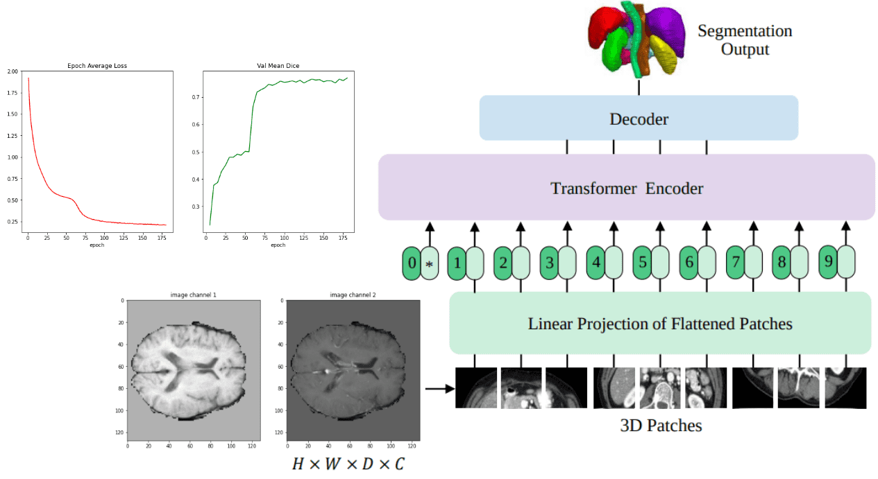
UNETR is the first successful transformer architecture for 3D medical image segmentation. In this blog post, I will try to match the results of a UNET model on the BRATS dataset, which contains 3D MRI brain images. Here is a high-level overview of UNETR that we will train in this tutorial:
 Source: UNETR: Transformers for 3D Medical Image Segmentation, Hatamizadeh et al.
To test my implementation I used an existing tutorial on a 3D MRI segmentation dataset. Thus, I have to give credit to the amazing open-source library of Nvidia called MONAI for providing the initial tutorial that I modified for educational purposes. If you are into medical imaging be sure to check out this awesome library and its tutorials.
Let's see the data first!
Update: Book release! Learn about “Deep learning in production” to serve your ML models to millions of users.
BRATS dataset
BRATS is a multi-modal large-scale 3D imaging dataset. It contains 4 3D volumes of MRI images captured under different modalities and setups. Here is a sample of the dataset. It is important to see that only the tumor is annotated. This makes things such as segmentation more difficult since the model has to localize on the tumor.
 Official data teaser image from the BRATS completion website
The image patches depict tumor categories as follows (from left to right):
Edema: The whole tumor (yellow) is usually visible in T2-FLAIR MRI image.
Non-enhancing solid core: The tumor core (red) visible in T2 MRI.
The enhancing tumor structures (light blue). Usually visible in T1Gd, surrounding the necrotic core (green).
The segmentations are combined to generate the final labels of the dataset.
With MONAI, loading a dataset from the medical imaging decathlon competition becomes trivial.
Data loading with MONAI and transformations
By utilizing the DecathlonDataset class of MONAI library one can load any of the 10 available datasets from the website. We will use Task01_BrainTumour in our case.
cache_num = 8from monai.apps import DecathlonDatasettrain_ds = DecathlonDataset(root_dir=root_dir,task="Task01_BrainTumour",transform=train_transform,section="training",download=True,num_workers=4,cache_num=cache_num,)train_loader = DataLoader(train_ds, batch_size=2, shuffle=True, num_workers=2)val_ds = DecathlonDataset(root_dir=root_dir,task="Task01_BrainTumour",transform=val_transform,section="validation",download=False,num_workers=4,cache_num=cache_num,)val_loader = DataLoader(val_ds, batch_size=2, shuffle=False, num_workers=2)
Imports and supporting functions can be found in the notebook. What’s crucial here is the transformation pipeline, which I guarantee is not an easy thing in 3D images. MONAI provides some functions to make a fast pipeline for the purpose of this tutorial. Details like the image orientation are left out of the tutorial on purpose.
Briefly, we will resample our images to a voxel size of 1.5, 1.5, and 2.0 mm in each dimension. Afterwards, we take random 3D sub-volumes of sizes 128, 128, 64. This of course needs to be applied to both the input image and the segmentation mask.
Then a couple of augmentations are applied such as randomly flipping the first axis, and rescaling the intensity (jittering).
The class ConvertToMultiChannelBasedOnBratsClassesd brings the labels to the format that we want.
from monai.transforms import (Activations,AsChannelFirstd,AsDiscrete,CenterSpatialCropd,Compose,LoadImaged,MapTransform,NormalizeIntensityd,Orientationd,RandFlipd,RandScaleIntensityd,RandShiftIntensityd,RandSpatialCropd,Spacingd,ToTensord,)roi_size=[128, 128, 64]pixdim=(1.5, 1.5, 2.0)class ConvertToMultiChannelBasedOnBratsClassesd(MapTransform):"""Convert labels to multi channels based on brats classes:label 1 is the peritumoral edemalabel 2 is the GD-enhancing tumorlabel 3 is the necrotic and non-enhancing tumor coreThe possible classes are TC (Tumor core), WT (Whole tumor)and ET (Enhancing tumor)."""def __call__(self, data):d = dict(data)for key in self.keys:result = []# merge label 2 and label 3 to construct TCresult.append(np.logical_or(d[key] == 2, d[key] == 3))# merge labels 1, 2 and 3 to construct WTresult.append(np.logical_or(np.logical_or(d[key] == 2, d[key] == 3), d[key] == 1))# label 2 is ETresult.append(d[key] == 2)d[key] = np.stack(result, axis=0).astype(np.float32)return dtrain_transform = Compose([# load 4 Nifti images and stack them togetherLoadImaged(keys=["image", "label"]),AsChannelFirstd(keys="image"),ConvertToMultiChannelBasedOnBratsClassesd(keys="label"),Spacingd(keys=["image", "label"],pixdim=pixdim,mode=("bilinear", "nearest"),),Orientationd(keys=["image", "label"], axcodes="RAS"),RandSpatialCropd(keys=["image", "label"], roi_size=roi_size, random_size=False),RandFlipd(keys=["image", "label"], prob=0.5, spatial_axis=0),NormalizeIntensityd(keys="image", nonzero=True, channel_wise=True),RandScaleIntensityd(keys="image", factors=0.1, prob=0.5),RandShiftIntensityd(keys="image", offsets=0.1, prob=0.5),ToTensord(keys=["image", "label"]),])val_transform = Compose([LoadImaged(keys=["image", "label"]),AsChannelFirstd(keys="image"),ConvertToMultiChannelBasedOnBratsClassesd(keys="label"),Spacingd(keys=["image", "label"],pixdim=pixdim,mode=("bilinear", "nearest"),),Orientationd(keys=["image", "label"], axcodes="RAS"),CenterSpatialCropd(keys=["image", "label"], roi_size=roi_size),NormalizeIntensityd(keys="image", nonzero=True, channel_wise=True),ToTensord(keys=["image", "label"]),])
It's always better to see the pipeline in action, by visualizing some slices from all the modalities. Below is a sample of our train data:
 Source: Image from the author based on the notebook
It can be observed that the tumor are not mutually exclusive. In this regard we expect the enhancing tumor and necrotic cells (rightmost segmentation map) to be the most difficult to predict.
The data and transformation pipeline are now all set. Let’s take a closer look at the model’s architecture.
Learn more about AI applied in medical imaging applications from the well-structured course AI for Medicine offered by Coursera.
The UNETR architecture
Here is the model architecture that incorporates transformers into the infamous UNET architecture:
 Source: UNETR: Transformers for 3D Medical Image Segmentation, Hatamizadeh et al.
Interestingly, I began to implement this model as in the paper figure depicted above. Later on, I discovered that it was already implemented in MONAI. After checking their code I found significant details missing. Conclusion: don’t trust the architecture images, they don’t include all the story on how to implement the paper. To see the implementation code, check out my implementation in the self-attention-cv library.
Now I can finally use my implementation of UNETR. I have created a small library that implements several self-attention blocks for computer vision and packs them in a pip-installable package. So now I only have to install my pip package that contains the model and voila:
$ pip install self-attention-cv==1.2.3
To initialize the model we need to provide the volume size, the input imaging modalities, the number of labels (output_dim) and several things regarding the vision transformer. Examples include embedding patch dimension, patch size, number of heads, normalization type etc.
from self_attention_cv import UNETRdevice = torch.device("cuda:0")num_heads = 10embed_dim= 512model = UNETR(img_shape=tuple(roi_size), input_dim=4, output_dim=3,embed_dim=embed_dim, patch_size=16, num_heads=num_heads,ext_layers=[3, 6, 9, 12], norm='instance',base_filters=16,dim_linear_block=2048).to(device)
I am still not sure why instance normalization works very well with UNETs and multi-model datasets, but it does! The point is that we have our 49.7 million parameter model ready to be trained.
We will use the DICE loss combined with cross-entropy, and make a simple training loop:
import torch.nn as nnfrom monai.losses import DiceLoss, DiceCELossloss_function = DiceCELoss(to_onehot_y=False, sigmoid=True)optimizer = torch.optim.AdamW(model.parameters(), lr=1e-4, weight_decay=1e-5)max_epochs = 180val_interval = 5best_metric = -1best_metric_epoch = -1epoch_loss_values = []for epoch in range(max_epochs):print(f"epoch {epoch + 1}/{max_epochs}")model.train()epoch_loss = 0step = 0for batch_data in train_loader:step += 1inputs, labels = (batch_data["image"].to(device),batch_data["label"].to(device),)optimizer.zero_grad()outputs = model(inputs)loss = loss_function(outputs, labels)loss.backward()optimizer.step()epoch_loss += loss.item()epoch_loss /= stepepoch_loss_values.append(epoch_loss)print(f"epoch {epoch + 1} average loss: {epoch_loss:.4f}")# Logging functionalities follow along in the notebook
Baseline comparison: UNET
Nonetheless, the biggest question here is how good this model can perform. For that reason, we need a strong baseline! What’s better than the well-configured UNET that is used in the initial tutorial?
I also compared my implementation with MONAI’s UNETR implementation. Why? Because there would be no meaning if I match the performance of the UNET baseline and still perform inferior to the official implementation. After all, I changed my code to reflect the architectural changes of the official code. And indeed I saw huge gains in performance compared to a simplistic implementation from the paper’s figure.
from monai.networks.nets import UNetmodel = UNet(dimensions=3,in_channels=4,out_channels=3,channels=(16, 32, 64, 128, 256),strides=(2, 2, 2, 2),num_res_units=2,).to(device)
Let's see the number's first:
| Model | epochs | Mean DICE coeff. |
| UNET (baseline) | 170 | 76.6 % |
| UNETR (self-attention-cv) | 180 | 76.9 % |
| UNETR (MONAI) | 180 | 76.1 % |
To track training we measure the training loss from both dice loss and cross-entropy. We also report the dice coefficients for the 3 labels (channels), namely Tumor Core (TC), Whole Tumor (WT), and Enhancing Tumor (EC).
Below you can see these metrics while training:
 Source: Image from the author based on the notebook
Finally, one can see the results by comparing the output segmentation map compared to the ground truth:
 Source: Image from the author based on the notebook
The channel of the necrotic area is omitted because this particular slice had almost no occurrences of this label. This illustration is only a middle slice of the 3D segmentation map, so it’s certainly not the whole picture. Still, it gives you the sense of how the trained model provides a more smothered version of the original label, which was annotated by an expert radiologist. Because as always neural networks love smooth optimization spaces.
Conclusion and concerns
I am not yet convinced by the performance of transformers in 3D medical imaging. I believe more advanced methods and other contributions will follow up. Yet I admit that it’s the first interesting work that challenges the well-configured UNET architectures, which are the go-to option in these tasks.
From the above analysis, I find it crucial to highlight also that the most important aspect to get a good performance, here Dice coefficient, is the data preprocessing and transformation pipelines. That’s exactly why I see limited innovation in the medical imaging world in terms of machine learning modelling, and more promising work on data processing optimization. That alone causes no issue at all, but it makes me very suspicious when a new paper comes out and claims a new architecture. Because the comparisons are often not fair in niche domains I happen to have worked on such as medical imaging.
As always, thanks for your interest in AI and stay tuned for more. We are proud to share with you our book on “Deep learning in production”, which teaches you how to put your model in production and scale it up. Community support (like social media sharing) is always appreciated.

* Disclosure: Please note that some of the links above might be affiliate links, and at no additional cost to you, we will earn a commission if you decide to make a purchase after clicking through.