Time for some hands-on tutorial on medical imaging. However, this time we will not use crazy AI but basic image processing algorithms. The goal is to familiarize the reader with concepts around medical imaging and specifically Computed Tomography (CT).
It is critical to understand how far one can go without deep learning, to understand when it’s best to use it. New practitioners tend to ignore that part, but medical image analysis is still 3D image processing.
I also include parts of the code to facilitate the understanding of my thought process.
The accompanying Google colab notebook can be found here to run the code shown in this tutorial. A Github repository is also available. Star our repo if you liked it!
To dive deeper into how AI is used in Medicine, you can’t go wrong with the AI for Medicine online course, offered by Coursera. If you want to focus on medical image analysis with deep learning, I highly recommend starting from the Pytorch-based Udemy Course.
We will start with the very basics of CT imaging. You may skip this section if you are already familiar with CT imaging.
CT imaging
Physics of CT Scans
Computed Tomography (CT) uses X-ray beams to obtain 3D pixel intensities of the human body. A heated cathode releases high-energy beams (electrons), which in turn release their energy as X-ray radiation. X-rays pass through human body tissues and hits a detector on the other side. A dense tissue (i.e. bones) will absorb more radiation than soft tissues (i.e. fat). When X-rays are not absorbed from the body (i.e. in the air region inside the lungs) and reach the detector we see them as black, similar to a black film. On the opposite, dense tissues are depicted as white.
In this way, CT imaging is able to distinguish density differences and create a 3D image of the body.

Here is a 1 min video I found very concise:
CT intensities and Hounsfield units
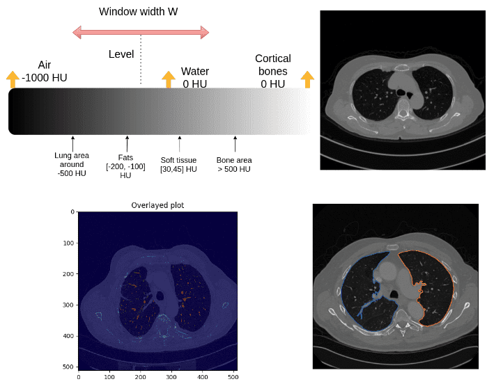
The X-ray absorption is measured in the Hounsfield scale. In this scale, we fix the Air intensity to -1000 and water to 0 intensity. It is essential to understand that Housenfield is an absolute scale, unlike MRI where we have a relative scale from 0 to 255.
The image illustrates some of the basic tissues and their corresponding intensity values. Keep in mind that the images are noisy. The numbers may slightly vary in real images.
 The Hounsfield scale. Image by Author.
Bones have high intensity. We usually clip the image to have an upper maximum range. For instance, the max value might be 1000, for practical reasons.
The problem: visualization libraries work on the scale [0,255]. It wouldn’t be very wise to visualize all the Hounsfield scale (from -1000 to 1000+ ) to 256 scales for medical diagnosis.
Instead, we limit our attention to different parts of this range and focus on the underlying tissues.
CT data visualization: level and window
The medical image convention to clip the Housenfield range is by choosing a central intensity, called level and a window, as depicted:

It is actually quite an ugly convention for computer scientists. We would just like the min and max of the range:
import matplotlib.pyplot as pltimport numpy as npdef show_slice_window(slice, level, window):"""Function to display an image sliceInput is a numpy 2D array"""max = level + window/2min = level - window/2slice = slice.clip(min,max)plt.figure()plt.imshow(slice.T, cmap="gray", origin="lower")plt.savefig('L'+str(level)+'W'+str(window))
If you are not convinced, the next image will convince you that the same CT image is more rich than a common image channel:
 Window and leveling in CT can give you quite different images. Image by Author.
For reference here is a list of visualization ranges:
| Region/Tissue | Window | Level |
| brain | 80 | 40 |
| lungs | 1500 | -600 |
| liver | 150 | 30 |
| Soft tissues | 250 | 50 |
| bone | 1800 | 400 |
Time to play!
Lung segmentation based on intensity values
We will not just segment the lungs but we will also find the real area in . To do that we need to find the real size of the pixel dimensions. Each image may have a different one (pixdim in the nifty header file). Let’s see the header file first:
import nibabel as nibct_img = nib.load(exam_path)print(ct_img.header)
Here I will show only some important fields of the header:
<class 'nibabel.nifti1.Nifti1Header'> object, endian='<'sizeof_hdr : 348dim : [ 2 512 512 1 1 1 1 1]datatype : int16bitpix : 16pixdim : [1. 0.78515625 0.78515625 1. 1. 1. 1. 1. ]srow_x : [ -0.78515625 0. 0. 206.60742 ]srow_y : [ 0. -0.78515625 0. 405.60742 ]srow_z : [ 0. 0. 1. -304.5]
For the record, srow_x, srow_y, srow_z is the affine matrix of the image. Bitpix is how many bits we use to represent each pixel intensity.
So let’s define a function that reads that information from the header file. Based on the nifty format each dimension in the nifty file has a pixel dimension. What we need is to find out the 2 dimension indices of the image and their respective pix dimensions.
Step 1: Find pixel dimensions to calculate the area in mm^2
def find_pix_dim(ct_img):"""Get the pixdim of the CT image.A general solution that gets the pixdim indicated from the image dimensions. From the last 2 image dimensions, we get their pixel dimension.Args:ct_img: nib imageReturns: List of the 2 pixel dimensions"""pix_dim = ct_img.header["pixdim"] # example [1,2,1.5,1,1]dim = ct_img.header["dim"] # example [1,512,512,1,1]max_indx = np.argmax(dim)pixdimX = pix_dim[max_indx]dim = np.delete(dim, max_indx)pix_dim = np.delete(pix_dim, max_indx)max_indy = np.argmax(dim)pixdimY = pix_dim[max_indy]return [pixdimX, pixdimY] # example [2, 1.5]
Step 2: Binarize image using intensity thresholding
We expect lungs to be in the Housendfield unit range of [-1000,-300]. To this end, we need to clip the image range to [-1000,-300] and binarize the values to 0 and 1, so we will get something like this:
 Image by Author
Step 3: Contour finding
Let's clarify what is a contour before anything else:
For computer vision, a contour is a set of points that describe a line or area. So for each detected contour we will not get a full binary mask but rather a set with a bunch of x and y values.
Ok, how can we isolate the desired area? Hmmm.. let’s think about it. We care about the lung regions that are shown on white. If we could find an algorithm to identify close sets or any kind of contours in the image that may help. After some search online, I found the marching squares method that finds constant valued contours in an image from skimage, called skimage.measure.find_contours().
After using this function I visualize the detected contours in the original CT image:
 Image by Author
Here is the function!
def intensity_seg(ct_numpy, min=-1000, max=-300):clipped = clip_ct(ct_numpy, min, max)return measure.find_contours(clipped, 0.95)
Step 4: Find the lung area from a set of possible contours
Note that I used a different image to show an edge case that the patient’s body is not a closed set of points. Ok, not exactly what we want, but let’s see if we could work that out.
Since we only care about the lungs we have to set some sort of constraints to exclude the unwanted regions.
To do so, I first extracted a convex polygon from the contour using scipy. After I assume 2 constraints:
The contour of the lungs must be a closed set (always true)
The contour must have a minimum volume of 2000 pixels to represent the lungs.
That may or may not include the body contour, resulting in more than 3 contours. When that happens the body is easily discarded by having the largest volume of the contour that satisfies the pre-described assumptions.
def find_lungs(contours):"""Chooses the contours that correspond to the lungs and the bodyFirst, we exclude non-closed sets-contoursThen we assume some min area and volume to exclude small contoursThen the body is excluded as the highest volume closed setThe remaining areas correspond to the lungsArgs:contours: all the detected contoursReturns: contours that correspond to the lung area"""body_and_lung_contours = []vol_contours = []for contour in contours:hull = ConvexHull(contour)# set some constraints for the volumeif hull.volume > 2000 and set_is_closed(contour):body_and_lung_contours.append(contour)vol_contours.append(hull.volume)# Discard body contourif len(body_and_lung_contours) == 2:return body_and_lung_contourselif len(body_and_lung_contours) > 2:vol_contours, body_and_lung_contours = (list(t) for t inzip(*sorted(zip(vol_contours, body_and_lung_contours))))body_and_lung_contours.pop(-1) # body is out!return body_and_lung_contours # only lungs left !!!
As an edge case, I am showing that the algorithm is not restricted to only two regions of the lungs. Inspect the blue contour below:
 Image by Author
Step 5: Contour to binary mask
Next, we save it as a nifty file so we need to convert the set of points to a lung binary mask. For this, I used the pillow python lib that draws a polygon and creates a binary image mask. Then I merge all the masks of the already found lung contours.
import numpy as npfrom PIL import Image, ImageDrawdef create_mask_from_polygon(image, contours):"""Creates a binary mask with the dimensions of the image andconverts the list of polygon-contours to binary masks and merges them togetherArgs:image: the image that the contours refer tocontours: list of contoursReturns:"""lung_mask = np.array(Image.new('L', image.shape, 0))for contour in contours:x = contour[:, 0]y = contour[:, 1]polygon_tuple = list(zip(x, y))img = Image.new('L', image.shape, 0)ImageDraw.Draw(img).polygon(polygon_tuple, outline=0, fill=1)mask = np.array(img)lung_mask += masklung_mask[lung_mask > 1] = 1 # sanity check to make 100% sure that the mask is binaryreturn lung_mask.T # transpose it to be aligned with the image dims
The desired lung area in is simply the number of nonzero elements multiplied by the two pixel dimensions of the corresponding image.
The lung areas are saved in a csv file along with the image name.
Finally, to save the mask as nifty I used the value of 255 for the lung area instead of 1 to be able to display in a nifty viewer. Moreover, I save the image with the affine transformation of the initial CT slice to be able to be displayed meaningfully (aligned without any rotation conflicts).
def save_nifty(img_np, name, affine):"""binary masks should be converted to 255 so it can be displayed in a nii viewerwe pass the affine of the initial image to make sure it exits in the sameimage coordinate spaceArgs:img_np: the binary maskname: output nameaffine: 4x4 np arrayReturns:"""img_np[img_np == 1] = 255ni_img = nib.Nifti1Image(img_np, affine)nib.save(ni_img, name + '.nii.gz')
Finally, I opened the mask with a common nifty viewer for Linux to validate that everything went ok. Here are snapshots for slice number 4:
 Image by Author
I used a free medical imaging viewer called Aliza on Linux.
Segment the main vessels and compute the vessels over lung area ratio
If there is a pixel with an intensity value over -500 HU inside the lung area then we will consider it as a vessel.
First, we do element-wise multiplication between the CT image and the lung mask to get only the lungs. Afterwards, we set the zeros that resulted from the element-wise multiplication to -1000 (AIR in HU) and finally keep only the intensities that are bigger than -500 as vessels.
def create_vessel_mask(lung_mask, ct_numpy, denoise=False):vessels = lung_mask * ct_numpy # isolate lung areavessels[vessels == 0] = -1000vessels[vessels >= -500] = 1vessels[vessels < -500] = 0show_slice(vessels)if denoise:return denoise_vessels(lungs_contour, vessels)show_slice(vessels)return vessels
One sample of this process can be illustrated below:
 The vessel mask with some noise. Image by Author.
Analyzing and improving the segmentation’s result
As you can see we have some parts of the contour of the lungs, which I believe we would like to avoid. To this end, I created a denoising function that considers the distance of the mask to all the contour points. If it is below 0.1, I set the pixel value to 0 and as a result exclude them from the detected vessels.
def denoise_vessels(lung_contour, vessels):vessels_coords_x, vessels_coords_y = np.nonzero(vessels) # get non zero coordinatesfor contour in lung_contour:x_points, y_points = contour[:, 0], contour[:, 1]for (coord_x, coord_y) in zip(vessels_coords_x, vessels_coords_y):for (x, y) in zip(x_points, y_points):d = euclidean_dist(x - coord_x, y - coord_y)if d <= 0.1:vessels[coord_x, coord_y] = 0return vessels
Below you can see the difference between the denoise image on the right and the initial mask:
 Image by Author
If we overlay the mask in the original CT image we get:
 Image by Author
def overlay_plot(im, mask):plt.figure()plt.imshow(im.T, 'gray', interpolation='none')plt.imshow(mask.T, 'jet', interpolation='none', alpha=0.5)
Now that we have the mask, the vessel area is computed similar to what I did for the lungs, by taking into account the individual image pixel dimension.
def compute_area(mask, pixdim):"""Computes the area (number of pixels) of a binary mask and multiplies the pixelswith the pixel dimension of the acquired CT imageArgs:lung_mask: binary lung maskpixdim: list or tuple with two valuesReturns: the lung area in mm^2"""mask[mask >= 1] = 1lung_pixels = np.sum(mask)return lung_pixels * pixdim[0] * pixdim[1]
The ratios are stored in a csv file in the notebook.
Conclusion and further readings
I believe that now you have a solid understanding of CT images and their particularities. We can do a lot of awesome things with such rich information of 3D images.
Support us by staring our project on GitHub. Finally, for more advanced tutorials see our medical imaging articles.
I have been asked for a large hands-on AI course. I am thinking of writing a book on medical imaging in 2021. Until then you can learn from the coursera course AI for Medicine.

* Disclosure: Please note that some of the links above might be affiliate links, and at no additional cost to you, we will earn a commission if you decide to make a purchase after clicking through.