What a rapid progress in ~8.5 years of deep learning! Back in 2012, Alexnet scored 63.3% Top-1 accuracy on ImageNet. Now, we are over 90% with EfficientNet architectures and teacher-student training.
If we plot the accuracy of all the reported works on Imagenet, we would get something like this:
 Source: Papers with Code - Imagenet Benchmark
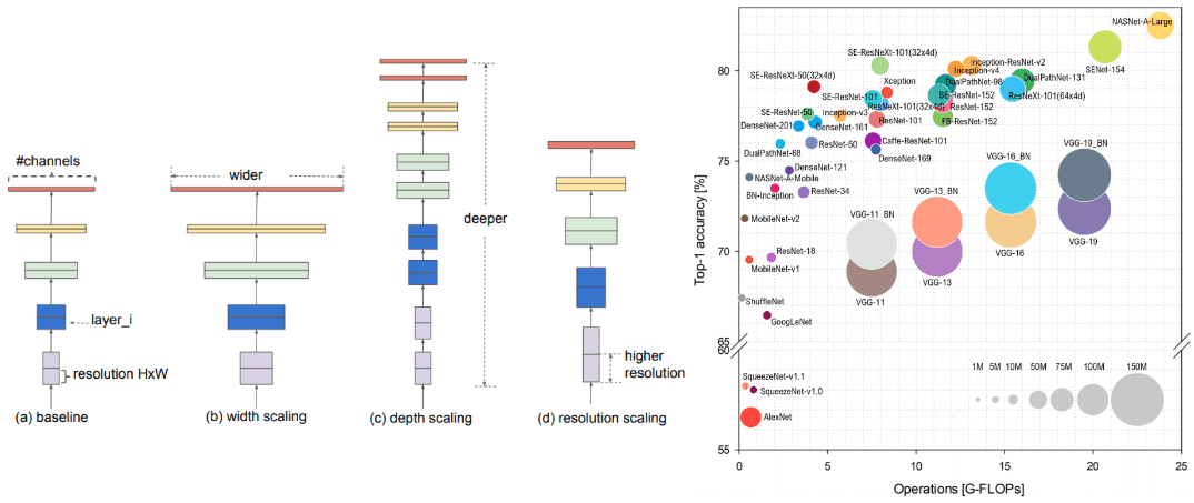
In this article, we will focus on the evolution of convolutional neural networks (CNN) architectures. Rather than reporting plain numbers, we will focus on the fundamental principles. To provide another visual overview, one could capture top-performing CNNs until 2018 in a single image:
 Overview of architectures until 2018. Source: Simone Bianco et al. 2018
Don’t freak-out. All the depicted architectures are based on the concepts that we will describe.
Note that, the FLoating point Operations Per second (FLOPs) indicate the complexity of the model, while on the vertical axis we have the Imagenet accuracy. The radius of the circle indicates the number of parameters.
From the above graph, it is evident that more parameters do not always lead to better accuracy. We will attempt to encapsulate a broader perspective on CNNs and see why this holds true.
If you want to understand how convolutions work from scratch, advise Andrew’s Ng course.
Terminology
But first, we have to define some terminology:
A wider network means more feature maps (filters) in the convolutional layers
A deeper network means more convolutional layers
A network with higher resolution means that it processes input images with larger width and depth (spatial resolutions). That way the produced feature maps will have higher spatial dimensions.
 Architecture scaling. Source: Mingxing Tan, Quoc V. Le 2019
Architecture engineering is all about scaling. We will thoroughly utilize these terms so be sure to understand them before you move on.
AlexNet: ImageNet Classification with Deep Convolutional Neural Networks (2012)
Alexnet [1] is made up of 5 conv layers starting from an 11x11 kernel. It was the first architecture that employed max-pooling layers, ReLu activation functions, and dropout for the 3 enormous linear layers. The network was used for image classification with 1000 possible classes, which for that time was madness. Now, you can implement it in 35 lines of PyTorch code:
class AlexNet(nn.Module):def __init__(self, num_classes: int = 1000) -> None:super(AlexNet, self).__init__()self.features = nn.Sequential(nn.Conv2d(3, 64, kernel_size=11, stride=4, padding=2),nn.ReLU(inplace=True),nn.MaxPool2d(kernel_size=3, stride=2),nn.Conv2d(64, 192, kernel_size=5, padding=2),nn.ReLU(inplace=True),nn.MaxPool2d(kernel_size=3, stride=2),nn.Conv2d(192, 384, kernel_size=3, padding=1),nn.ReLU(inplace=True),nn.Conv2d(384, 256, kernel_size=3, padding=1),nn.ReLU(inplace=True),nn.Conv2d(256, 256, kernel_size=3, padding=1),nn.ReLU(inplace=True),nn.MaxPool2d(kernel_size=3, stride=2),)self.avgpool = nn.AdaptiveAvgPool2d((6, 6))self.classifier = nn.Sequential(nn.Dropout(),nn.Linear(256 * 6 * 6, 4096),nn.ReLU(inplace=True),nn.Dropout(),nn.Linear(4096, 4096),nn.ReLU(inplace=True),nn.Linear(4096, num_classes),)def forward(self, x: torch.Tensor) -> torch.Tensor:x = self.features(x)x = self.avgpool(x)x = torch.flatten(x, 1)x = self.classifier(x)return x
It was the first convolutional model that was successfully trained on Imagenet and for that time, it was much more difficult to implement such a model in CUDA. Dropout is heavily used in the enormous linear transformations to avoid overfitting. Before 2015-2016 that auto-differentiation came out, it took months to implement backprop on the GPU.
VGG (2014)
The famous paper “Very Deep Convolutional Networks for Large-Scale Image Recognition” [2] made the term deep viral. It was the first study that provided undeniable evidence that simply adding more layers increases the performance. Nonetheless, this assumption holds true up to a certain point. To do so, they use only 3x3 kernels, as opposed to AlexNet. The architecture was trained using 224 × 224 RGB images.
The main principle is that a stack of three conv. layers are similar to a single layer. And maybe even better! Because they use three non-linear activations in between (instead of one), which makes the function more discriminative.
Secondly, this design decreases the number of parameters. Specifically, you need weights, compared to a conv. layer that would require parameters (81% more).
Intuitively, it can be regarded as a regularisation on the conv. filters, constricting them to have a 3x3 non-linear decomposition.
Finally, it was the first architecture that normalization started to become quite an issue.
Nevertheless, pretrained VGGs are still used for feature matching loss in Generative adversarial Networks, as well as neural style transfer and feature visualizations.
In my humble opinion, it is very interesting to inspect the features of a convnet with respect to the input, as shown in the following video:
Finally to get a visual comparison next to Alexnet:
 Source: Standford 2017 Deep Learning Lectures: CNN architectures
InceptionNet/GoogleNet (2014)
After VGG, the paper “Going Deeper with Convolutions” [3] by Christian Szegedy et al. was a huge breakthrough.
Motivation: Increasing the depth (number of layers) is not the only way to make a model bigger. What about increasing both the depth and width of the network while keeping computations to a constant level?
This time the inspiration comes from the human visual system, wherein information is processed at multiple scales and then aggregated locally [3]. How to achieve this without a memory explosion?
The answer is with convolutions! The main purpose is dimension reduction, by reducing the output channels of each convolution block. Then we can process the input with different kernel sizes. As long as the output is padded, it is the same as in the input.
To find the appropriate padding with single stride convs without dilation, padding and kernel are defined so that (input and output spatial dims):
, which means that . In Keras you simply specify padding=’same’. This way, we can concatenate features convolved with different kernels.
Then we need the convolutional layer to ‘project’ the features to fewer channels in order to win computational power. And with these extra resources, we can add more layers. Actually, the convs work similar to a low dimensional embedding.
For a quick overview on 1x1 convs advise this video from the famous Coursera course:
This in turn allows to not only increase the depth, but also the width of the famous GoogleNet by using Inception modules. The core building block, called the inception module, looks like this:
 Szegedy et al. 2015. Source
The whole architecture is called GoogLeNet or InceptionNet. In essence, the authors claim that they try to approximate a sparse convnet with normal dense layers (as shown in the figure).
Why? Because they believe that only a small number of neurons are effective. This comes in line with the Hebbian principle: “Neurons that fire together, wire together”.
Moreover, it uses convolutions of different kernel sizes (, , ) to capture details at multiple scales.
In general, a larger kernel is preferred for information that resides globally, and a smaller kernel is preferred for information that is distributed locally.
Besides, convolutions are used to compute reductions before the computationally expensive convolutions (3×3 and 5×5).
The InceptionNet/GoogLeNet architecture consists of 9 inception modules stacked together, with max-pooling layers between (to halve the spatial dimensions). It consists of 22 layers (27 with the pooling layers). It uses global average pooling after the last inception module.
I wrote a very simple implementation of an Inception block that might clarify things out:
import torchimport torch.nn as nnclass InceptionModule(nn.Module):def __init__(self, in_channels, out_channels):super(InceptionModule, self).__init__()relu = nn.ReLU()self.branch1 = nn.Sequential(nn.Conv2d(in_channels, out_channels=out_channels, kernel_size=1, stride=1, padding=0),relu)conv3_1 = nn.Conv2d(in_channels, out_channels=out_channels, kernel_size=1, stride=1, padding=0)conv3_3 = nn.Conv2d(out_channels, out_channels, kernel_size=3, stride=1, padding=1)self.branch2 = nn.Sequential(conv3_1, conv3_3,relu)conv5_1 = nn.Conv2d(in_channels, out_channels=out_channels, kernel_size=1, stride=1, padding=0)conv5_5 = nn.Conv2d(out_channels, out_channels, kernel_size=5, stride=1, padding=2)self.branch3 = nn.Sequential(conv5_1,conv5_5,relu)max_pool_1 = nn.MaxPool2d(kernel_size=3, stride=1, padding=1)conv_max_1 = nn.Conv2d(in_channels, out_channels=out_channels, kernel_size=1, stride=1, padding=0)self.branch4 = nn.Sequential(max_pool_1, conv_max_1,relu)def forward(self, input):output1 = self.branch1(input)output2 = self.branch2(input)output3 = self.branch3(input)output4 = self.branch4(input)return torch.cat([output1, output2, output3, output4], dim=1)model = InceptionModule(in_channels=3,out_channels=32)inp = torch.rand(1,3,128,128)print(model(inp).shape)
torch.Size([1, 128, 128, 128])
You can find the google colab for the above code here.
Of course, you can add a normalization layer before the activation function. But since normalization techniques were not very well established the authors introduced two auxiliary classifiers. The reason: the vanishing gradient problem).
Inception V2, V3 (2015)
Later on, in the paper “Rethinking the Inception Architecture for Computer Vision” the authors improved the Inception model based on the following principles:
Factorize 5x5 and 7x7 (in InceptionV3) convolutions to two and three 3x3 sequential convolutions respectively. This improves computational speed. This is the same principle as VGG.
They used spatially separable convolutions. Simply, a 3x3 kernel is decomposed into two smaller ones: a 1x3 and a 3x1 kernel, which are applied sequentially.
The inception modules became wider (more feature maps).
They tried to distribute the computational budget in a balanced way between the depth and width of the network.
They added batch normalization.
Later versions of the inception model are InceptionV4 and Inception-Resnet.
ResNet: Deep Residual Learning for Image Recognition (2015)
All the predescribed issues such as vanishing gradients were addressed with two tricks:
batch normalization and
short skip connections
Instead of , we ask them model to learn the difference (residual) , which means will be the residual part [4].
 Source: Standford 2017 Deep Learning Lectures: CNN architectures
With that simple but yet effective block, the authors designed deeper architectures ranging from 18 (Resnet-18) to 150 (Resnet-150) layers.
For the deepest models they adopted 1x1 convs, as illustrated on the right:
 Image by Kaiming He et al. 2015. Source:Deep Residual Learning for Image Recognition
The bottleneck layers (1×1) layers first reduce and then restore the channel dimensions, leaving the 3×3 layer with fewer input and output channels.
Overall, here is a sketch of the whole architecture:
For more details, you can watch an awesome video from Henry AI Labs on ResNets:
You can play around with a bunch of ResNets by directly importing them from torchvision:
import torchvisionpretrained = True# A lot of choices :Pmodel = torchvision.models.resnet18(pretrained)model = torchvision.models.resnet34(pretrained)model = torchvision.models.resnet50(pretrained)model = torchvision.models.resnet101(pretrained)model = torchvision.models.resnet152(pretrained)model = torchvision.models.wide_resnet50_2(pretrained)model = torchvision.models.wide_resnet101_2(pretrained)
Try them out!
DenseNet: Densely Connected Convolutional Networks (2017)
Skip connections are a pretty cool idea. Why don’t we just skip-connect everything?
Densenet is an example of pushing this idea into the extremity. Of course, the main difference with ResNets is that we will concatenate instead of adding the feature maps.
Thus, the core idea behind it is feature reuse, which leads to very compact models. As a result it requires fewer parameters than other CNNs, as there are no repeated feature-maps.
Ok, why not? Hmmm… there are two concerns here:
The feature maps have to be of the same size.
The concatenation with all the previous feature maps may result in memory explosion.
To address the first issue we have two solutions:
a) use conv layers with appropriate padding that maintain the spatial dims or
b) use dense skip connectivity only inside blocks called Dense Blocks.
An exemplary image is shown below:
 Image by author. The Dense block is taken from Gao Huang et al. Source: Densenet
The transition layer can down-sample the image dimensions with average pooling.
To address the second concern which is memory explosion, the feature maps are reduced (kind of compressed) with 1x1 convs. Notice that I used K in the diagram, but densenet uses
Furthermore, they add a dropout layer with p=0.2 after each convolutional layer when no data augmentation is used.
Growth rate
More importantly, there is another parameter that controls the number of feature maps of the total architecture. It is the growth rate. It specifies the output features of each extra dense conv layer. Given initial feature maps and growth rate, one can calculate the number of input feature maps of each layer as . In frameworks, the number k is in multiples of 4, called bottleneck size (bn_size).
Finally, I am referencing here DenseNet’s most important arguments from torchvision as a sum up:
import torchvisionmodel = torchvision.models.DenseNet(growth_rate = 16, # how many filters to add each layer (`k` in paper)block_config = (6, 12, 24, 16), # how many layers in each pooling blocknum_init_features = 16, # the number of filters to learn in the first convolution layer (k0)bn_size= 4, # multiplicative factor for number of bottleneck (1x1 cons) layersdrop_rate = 0, # dropout rate after each dense conv layernum_classes = 30 # number of classification classes)print(model) # see snapshot below
Inside the “dense” layer (denselayer5 and 6 in the snapshot) there is a bottleneck (1x1) layer that reduces the channels to in our case. Otherwise, the number of input channels would explode. As demonstrated below each layer adds up channels.

In practice, I have found the DenseNet-based models quite slow to train but with very few parameters compared to models that perform competitively, due to feature reuse.
Even though DenseNet was proposed for image classification, it has been used in various applications in domains where feature reusability is more crucial (i.e. segmentation and medical imaging application). The pie diagram borrowed from Papers with Code illustrates this:
 Image by Papers with Code
After DenseNet in 2017, I only found interesting the HRNet architecture up until 2019 when EfficientNet came out!
Big Transfer (BiT): General Visual Representation Learning (2020)
Even though many variants of ResNet have been proposed, the most recent and famous one is BiT. Big Transfer (BiT) is a scalable ResNet-based model for effective image pre-training [5].
They developed 3 BiT models (small, medium and large) based on ResNet152. For the large variation of BiT they used ResNet152x4, which means that each layer has 4 times more channels. They pretrained that model once in far more bigger datasets than imagenet. The largest model was trained on the insanely large JFT dataset, which consists of 300M labeled images.
The major contribution in the architecture is the choice of normalization layers. To this end, the authors replaced batch normalization (BN) with group normalization (GN) and weight standardization (WS).
 Image by Lucas Beyer and Alexander Kolesnikov. Source
Why? Because first BN’s parameters (means and variances) need adjustment between pre-training and transfer. On the other hand, GN doesn’t depend on any parameter states. Another reason is that BN uses batch-level statistics, which become unreliable for distributed training in small devices like TPU’s. A 4K batch distributed across 500 TPU’s means 8 batches per worker, which does not give a good estimation of the statistics. By changing the normalization technique to GN+WS they avoid synchronization across workers.
Obviously, scaling to larger datasets come hand in hand with the model size.
 Performance with more and and multiple models. Source: Alexander Kolesnikov et al. 2020
In this figure, the importance of scaling up the architecture in parallel with the data is illustrated. ILSVER is the Imagenet dataset with 1M images, ImageNet-21K has approximately 14M images and JFT 300M!
Finally, such large pretrained models can be fine-tuned to very small datasets and achieve very good performance.
 Performance of BiT models with limited data for fine tuning. Source: Alexander Kolesnikov et al. 2020
With 5 examples per class on ImageNet a widened by a factor of 3, a ResNet-50 (x3) pretrained on JFT achieves similar performance to AlexNet!
EfficientNet: Rethinking Model Scaling for Convolutional Neural Networks (2019)
EfficientNet is all about engineering and scale. It proves that if you carefully design your architecture you can achieve top results with reasonable parameters.
 Image by Mingxing Tan and Quoc V. Le 2020. Source: EfficientNet: Rethinking Model Scaling for Convolutional Neural Networks
The graph demonstrates the ImageNet Accuracy VS model parameters.
It’s incredible that EfficientNet-B1 is 7.6x smaller and 5.7x faster than ResNet-152.
Individual upscaling
Let’s understand how this is possible.
With more layers (depth) one can capture richer and more complex features, but such models are hard to train (due to the vanishing gradients)
Wider networks are much easier to train. They tend to be able to capture more fine-grained features but saturate quickly.
By training with higher resolution images, convnets are in theory able to capture more fine-grained details. Again, the accuracy gain diminishes for quite high resolutions
Instead of finding the best architecture, the authors proposed to start with a relatively small baseline model and gradually scale it.
That narrows down the design space. To constrain the design space even further, the authors restrict all the layers to uniform scaling with a constant ratio. This way, we have a more tractable optimization problem. And finally, one has to respect the maximum number of memory and FLOPs of our infrastructure.
This is nicely demonstrated in the following diagrams:
 Image by Mingxing Tan and Quoc V. Le 2020. Source: EfficientNet: Rethinking Model Scaling for Convolutional Neural Networks
is the width, the depth, and the resolution scaling factors. By scaling one only one of them will saturate at a point. Can we do better?
Compound scaling
So let’s instead scale up network depth (more layers), width (more channels per layer), resolution (input image) simultaneously. This is known as compound scaling.
To do so, we have to balance all the aforementioned dimensions during scaling. Here it gets exciting.
Such that: , given all
Now controls all the desired dimensions and scales them together but not equally. tell us how to distribute the additional resources to the network.
Notice anything strange? and are squared in the constraint.
The reason is simple: doubling network depth will double FLOPS, but doubling width or input resolution will increase FLOPS by four times. In this way, we are resembling the convolution, which is the fundamental building block.
The baseline architecture was found using neural architecture search so that it optimizes both accuracy and FLOPS, called EfficientNet-B0.
Ok cool. What’s left is to define and .
Fix , assume that twice more resources are available, and do a grid search of . The best acquired values for EfficientNet-B0 are
Fix and scale up with respect to the hardware (FLOPs + memory)
In my opinion, the most intuitive way to understand the effectiveness of compound scaling is on par with individual scaling of the same baseline model (EfficientNet-B0) on ImageNet:
 Image by Mingxing Tan and Quoc V. Le 2020. Source: EfficientNet: Rethinking Model Scaling for Convolutional Neural Networks
Self-training with Noisy Student improves ImageNet classification (2020)
Shortly after, an iterative semi-supervised method was used. It improved Efficient-Net’s performance significantly with 300M unlabeled images. The author called the training scheme “Noisy Student Training” [8]. It consists of two neural networks, called the teacher and the student. The iterative training scheme can be described in 4 steps:
Train a teacher model on labeled images,
Use the teacher to generate labels on 300M unlabeled images (pseudo-labels)
Train a student model on the combination of labeled images and pseudo labeled images.
Iterate from step 1, by treating the student as a teacher. Re-infer the unlabeled data and train a new student from scratch.
The new student model is normally larger than the teacher so it can benefit from a larger dataset. Furthermore, significant noise is added to train the student model so it is forced to learn harder from the pseudo labels.
The pseudo-labels are usually soft (a continuous distribution) instead of hard (a one-hot encoding).
Moreover, different techniques such as dropout and stochastic depth are used to train the new student [8].
 Image by Qizhe Xie et al. Source: Self-training with Noisy Student improves ImageNet classification
In step 3, we jointly train the model with both labeled and unlabeled data. The unlabeled batch size is set to 14 times the labeled batch size on the first iteration, and 28 times in the second iteration.
Meta Pseudo-Labels (2021)
Motivation: If the pseudo labels are inaccurate, the student will NOT surpass the teacher. This is called confirmation bias in pseudo-labeling methods.
High-level idea: Design a feedback mechanism to correct the teacher’s bias.
The observation comes from how pseudo labels affect the student’s performance on the labeled dataset. The feedback signal is the reward to train the teacher, similarly to reinforcement learning techniques.
 Hieu Pham et al 2020. Source: Meta Pseudo Labels
This way, the teacher and student are jointly trained. The teacher learns from the reward signal how well the student performs on a batch of images coming from the labeled dataset.
Sum up
That’s a lot of convnets out there! We can summarize them by looking at this table:
| Model name | Number of parameters [Millions] | ImageNet Top 1 Accuracy | Year |
| AlexNet | 60 M | 63.3 % | 2012 |
| Inception V1 | 5 M | 69.8 % | 2014 |
| VGG 16 | 138 M | 74.4 % | 2014 |
| VGG 19 | 144 M | 74.5 % | 2014 |
| Inception V2 | 11.2 M | 74.8 % | 2015 |
| ResNet-50 | 26 M | 77.15 % | 2015 |
| ResNet-152 | 60 M | 78.57 % | 2015 |
| Inception V3 | 27 M | 78.8 % | 2015 |
| DenseNet-121 | 8 M | 74.98 % | 2016 |
| DenseNet-264 | 22M | 77.85 % | 2016 |
| BiT-L (ResNet) | 928 M | 87.54 % | 2019 |
| NoisyStudent EfficientNet-L2 | 480 M | 88.4 % | 2020 |
| Meta Pseudo Labels | 480 M | 90.2 % | 2021 |
You can notice how compact DenseNet models are. Or how huge the state-of-the-art EfficientNet is. More parameters do not always guarantee more accuracy as you can see with BiT and VGG.
In this article, we provided some intuition behind the most famous deep learning architectures. Having that said, the only way to move on is to practice! Import a model from torchvision and finetune it on your data. Does it provide better accuracy than training from scratch?
What's next? A solid and holistic approach to computer vision systems with Deep Learning. Give it a shot! Use the discount code aisummer35 to get an exclusive 35% discount from your favorite AI blog. Use the discount code aisummer35 to get an exclusive 35% discount from your favorite AI blog. If your prefer a visual course, the Convolutional Neural Networks by Andrew Ng is by far the best one
References
[1] Krizhevsky, A., Sutskever, I., & Hinton, G. E. (2017). Imagenet classification with deep convolutional neural networks. Communications of the ACM, 60(6), 84-90.
[2] Simonyan, K., & Zisserman, A. (2014). Very deep convolutional networks for large-scale image recognition. arXiv preprint arXiv:1409.1556.
[3] Szegedy, C., Liu, W., Jia, Y., Sermanet, P., Reed, S., Anguelov, D., ... & Rabinovich, A. (2015). Going deeper with convolutions. In Proceedings of the IEEE conference on computer vision and pattern recognition (pp. 1-9).
[4] He, K., Zhang, X., Ren, S., & Sun, J. (2016). Deep residual learning for image recognition. In Proceedings of the IEEE conference on computer vision and pattern recognition (pp. 770-778).
[5] Kolesnikov, A., Beyer, L., Zhai, X., Puigcerver, J., Yung, J., Gelly, S., & Houlsby, N. (2019). Big transfer (bit): General visual representation learning. arXiv preprint arXiv:1912.11370, 6(2)
[6] Huang, G., Liu, Z., Van Der Maaten, L., & Weinberger, K. Q. (2017). Densely connected convolutional networks. In Proceedings of the IEEE conference on computer vision and pattern recognition (pp. 4700-4708).
[7] Tan, M., & Le, Q. V. (2019). Efficientnet: Rethinking model scaling for convolutional neural networks. arXiv preprint arXiv:1905.11946.
[8] Xie, Q., Luong, M. T., Hovy, E., & Le, Q. V. (2020). Self-training with noisy student improves imagenet classification. In Proceedings of the IEEE/CVF Conference on Computer Vision and Pattern Recognition (pp. 10687-10698).
[9] Pham, H., Xie, Q., Dai, Z., & Le, Q. V. (2020). Meta pseudo labels. arXiv preprint arXiv:2003.10580.
[10] Szegedy, C., Vanhoucke, V., Ioffe, S., Shlens, J., & Wojna, Z. (2016). Rethinking the inception architecture for computer vision. In Proceedings of the IEEE conference on computer vision and pattern recognition (pp. 2818-2826).

* Disclosure: Please note that some of the links above might be affiliate links, and at no additional cost to you, we will earn a commission if you decide to make a purchase after clicking through.