Recurrent neural networks: building a custom LSTM cell

An infinite amount of times I have found myself in desperate situations because I had no idea what was happening under the hood. And, for a lot of people in the computer vision community, recurrent neural networks (RNNs) are like this. More or less, another black box in the pile.

However, in this tutorial, we will attempt to open the RNN magic black box and unravel its mysteries!

Even though I have come across hundreds of tutorials on LSTM’s out there, I felt there was something missing. Therefore, I honestly hope that this tutorial serves as a modern guide to RNNs. We try to deal with multiple details of practical nature. To this end, we will build upon their fundamental concepts.

The vast application field of RNN’s includes sequence prediction, activity recognition, video classification as well as a variety of natural language processing tasks. After a careful inspection of the equations, we will build our own LSTM cell to validate our understanding. Finally, we will make some associations with convolutional neural networks to maximize our comprehension. Accompanying code for this tutorial can be found here.

It is true that by the moment you start to read about RNN’s, especially with a computer vision background, concepts misleadings start to arise. Less literally:

“Backpropagation with stochastic gradient descent (SGD) does not magically make your network work. Batch normalization does not magically make it converge faster. Recurrent Neural Networks (RNNs) don’t magically let you “plug in” sequences. (...) If you insist on using the technology without understanding how it works you are likely to fail.” ~ Andrey Karpathy (Director of AI at Tesla)

The abstraction of RNN's implementations doesn't allow users to understand how we deal with the time dimension in sequences! However, by understanding how it works you can write optimized code and practice extensibility, in a way that you weren't confident enough to do before.

Finally, a more holistic approach in RNN’s can be found on Sequence models from the Deep Learning specialization course offered by Coursera.

A simple RNN cell

Recurrent cells are neural networks (usually small) for processing sequential data. As we already know, convolutional layers are specialized for processing grid-structured values (i.e. images). On the contrary, recurrent layers are designed for processing long sequences, without any extra sequence-based design choice [1].

One can achieve this by connecting the timesteps’ output to the input! This is called sequence unrolling. By processing the whole sequence, we have an algorithm that takes into account the previous states of the sequence. In this manner, we have the first notion of memory (a cell)! Let’s look at it:

Visualization is borrowed from Wiki

The majority of common recurrent cells can also process sequences of variable length. This is really important for many applications such as videos, that contain a different number of images. One can view the RNN cell as a common neural network with shared weights for the multiple timesteps. With this modification, the weights of the cell now have access to the previous states of the sequence.

But how can we possibly train such sequential models?

What is Back-propagation through time?

Most practitioners with computer vision background have little idea of what recurrency means. And it is indeed difficult to understand. Because the frameworks assume that you already know how it works. However, if you want to find an efficient solution to your problem, you should carefully design your architecture based on the problem.

The magic of RNN networks that nobody sees is the input unrolling. The latter means that given a sequence of length N, you process the input into timesteps.

We choose to model the time dimension with RNN’s, because we want to learn temporal and often long-term dependencies.

Right now, it is true that convolutions cannot handle because they have a finite receptive field. Note that, in theory, you can apply a recurrent model in any dimension.

In terms of training an RNN model, the issue is that now we have a time-sequence. That’s why input unrolling is the only way we can make backpropagation work!

So, how can you learn a time-sequence? Ideally, we would like the memory (parameters) of the cells to have taken into account all the input sequences. Otherwise, we would not be able to learn the desired mapping. In essence, backpropagation requires a separate layer for each time step with the same weights for all layers (input unrolling)! The following image helps to understand this tricky idea.

Source: O’Reilly: hands-on-reinforcement-learning](Source: O’Reilly: hands-on-reinforcement-learning)

Backpropagation through time was created based on the pre-described observation. So, based on the chunked (unrolled) input, we can calculate a different loss per timestep. Then, we can backpropagate the error of multiple losses to the memory cells. In this direction, one can compute the gradients from multiple paths (timesteps) that then are added to calculate the final gradient. For this reason, we may use different optimizers or normalization methods in recurrent architectures.

In other words, we represent the RNN as a repeated (feedforward) network. More importantly, the time and space complexity to produce the output of the RNN is asymptotically linear to the input length (timesteps). This practical bottleneck introduces the computational limit of training really large sequences.

In fact, a similar idea is implemented in practice when you have a small GPU and you want to train your model with a bigger batch size than your memory supports. You perform forward propagation with the first batch and calculate the loss. Afterwards, you repeat the same thing with the second batch and average the losses from different batches. In this way, gradients are accumulated. With this trick of the low budget machine learners, you basically perform a similar operation to backpropagation through time. Finally, siamese networks with shared weights also roughly exploit this concept.

Let’s now see the inside of an LSTM [5] cell.

LSTM: Long-short term memory cells

Why LSTM?

One of the most fundamental works in the field was by Greff et al. 2016 [4]. Briefly, they showed that the proposed variations of RNN do not provide any significant improvement in a large scale study compared to LSTM. Therefore, LSTM is the dominant architecture in RNNs. That’s why we will focus on this RNN variation.

How LSTM works?

We can write forever about what an LSTM cell is, or how it is used in many applications. However, the language of mathematics makes this world beautiful and compact for us. Let’s see the math. Don’t be scared! We will slowly clarify every term, by inspecting every equation separately.

Before we begin, note that in all the equations, the weight matrices (W) are indexed, with the first index being the vector that they process, while the second index refers to the representation (i.e. input gate, forget gate).

To avoid confusion and maximize understanding, we will use the common notation: matrices are depicted with capital bold letters while vectors with non-capital bold letters. For the element-wise multiplication, I used the dot with the outer circle symbol, referred to as the Hadamard product [9] in the bibliography.

Equations of the LSTM cell

For $\textbf{x}_t \in R^{N}$ , where N is the feature length of each timestep, while $\textbf{i}_t,\textbf{f}_t,\textbf{o}_t,\textbf{h}_t,\textbf{h}_{t-1},\textbf{c}_t,\textbf{c}_{t-1},\textbf{b} \in R^{H}$ , where H is the hidden state dimension, the LSTM equations are the following:

\textbf{i}_t = \sigma( \textbf{W}_{xi} \textbf{x}_t + \textbf{W}_{hi} \textbf{h}_{t-1} + \textbf{W}_{ci} \textbf{c}_{t-1} + \textbf{b}_i) \quad\quad(1)

\textbf{f}_t = \sigma( \textbf{W}_{xf} \textbf{x}_t + \textbf{W}_{hf} \textbf{h}_{t-1} + \textbf{W}_{cf} \textbf{c}_{t-1} + \textbf{b}_f) \quad\quad(2)

\textbf{c}_t = \textbf{f}_t \odot \textbf{c}_{t-1} + \textbf{i}_t \odot tanh( \textbf{W}_{xc} x_t + \textbf{W}_{hc} \textbf{h}_{t-1} + \textbf{b}_c ) \quad\quad(3)

\textbf{o}_t = \sigma( \textbf{W}_{xo} \textbf{x}_t + \textbf{W}_{h0} \textbf{h}_{t-1} + \textbf{W}_{co} \textbf{c}_{t} + \textbf{b}_o) \quad\quad(4)

\textbf{h}_t = \textbf{o}_t \odot tanh(\textbf{c}_t) \quad\quad(5)

The LSTM cell equations were written based on Pytorch documentation because you will probably use the existing layer in your project. In the original paper, $\textbf{c}_{t-1}$ is included in the Equation (1) and (2), but you can omit it. For consistency reasons with the Pytorch docs, I will not include these computations in the code. For the record, these kind of connections are called peephole connection in the literature.

Equation 1: the input gate

\textbf{i}_t = \sigma( \textbf{W}_{xi} \textbf{x}_t + \textbf{W}_{hi} \textbf{h}_{t-1} + \textbf{W}_{ci} \textbf{c}_{t-1} + \textbf{b}_i)

The depicted weight matrices represent the memory of the cell. You see the input $\textbf{x}_t$ is in the current input timestep, while h and c are indexed with the previous timestep. Every matrix W is a linear layer (or simply a matrix multiplication). This equation enables us to the following:

a) take multiple linear combinations of x,h,c, and

b) match the dimensionality of input x to the one of h and c.

The dimensionalities of h and c are basically the hidden states parameter in a deep learning framework such as PyTorch (LSTM Pytorch layer documentation). For the old-school readers, hidden states were referenced in older literature as neurons, but now this term is deprecated.

Moving on, the bias term is part of the linear layer and is simply a trainable vector that is added. The output is also in the dimensionality of the hidden and context/cell vector [1]. Finally, after the 3 linear layers from different inputs, we have a non-linear activation function to introduce non-linearities, which enables the learning of more complex representations. In this case, the sigmoid function is usually used.

Equation 2: the forget gate

\textbf{f}_t = \sigma( \textbf{W}_{xf} \textbf{x}_t + \textbf{W}_{hf} \textbf{h}_{t-1} + \textbf{W}_{cf} \textbf{c}_{t-1} + \textbf{b}_f)

Simply, equation 2 is exactly the same thing as equation 1. However, note that the weight matrices are different this time. This means that we get a different set of linear combinations, that represent different things! The equations might be the same, however, we want to model different things, as you will see.

Equation 3: the new cell/context vector

Notice that I use cell or context vector interchangeably.

\textbf{c}_t = \textbf{f}_t \odot \textbf{c}_{t-1} + \textbf{i}_t \odot tanh( \textbf{W}_{xc} x_t + \textbf{W}_{hc} \textbf{h}_{t-1} + \textbf{b}_c ) \quad\quad(3)

We have already learned a representation that corresponds to “forget”, as well as for modeling the “input vector”, f and i, respectively. Let’s keep them aside and first inspect the $tanh$ parenthesis.

Here, we have another linear combination of the input and hidden vector, which is again totally different! This term is the new cell information, passed by the tanh function so as to introduce non-linearity and stabilize training.

But we don’t want to simply update the cell with the new states. Intuitively, we want to take into account previous states; that’s why we designed RNNs anyway! This is where the calculated input gate vector i comes into play. We filter the new cell info by applying an element-wise multiplication with the input gate vector i (similar to a filter in signal processing).

The forget gate vector comes into play now. Instead of just adding the filtered input info, we first perform an element-wise vector multiplication with the previous context vector. To this end, we would like the model to mimic the forgetting notion of humans as a multiplication filter.

By adding the previously described term in the $tanh$ parenthesis, we get the new cell state, as shown in Equation 3.

But what about the output of the LSTM [5] cell in a single timestep?

Equation 4, the almost new output

\textbf{o}_t = \sigma( \textbf{W}_{xo} \textbf{x}_t + \textbf{W}_{h0} \textbf{h}_{t-1} + \textbf{W}_{co} \textbf{c}_{t} + \textbf{b}_o)

It’s simple! Let’s just take another linear combination! This time, of our 3 vectors $x_t, h_(t-1), c_t$ , while we add another non-linear function in the end. Note that, we will now use the calculated new cell state (c_t) as opposed to equations 1 and 2. We have almost calculated the desired output vector $o_t$ of a single cell in a particular timestep.

Equation 5, the new context

\textbf{h}_t = \textbf{o}_t tanh(\textbf{c}_t) \quad\quad(5)

Note that the title in equation 4 was the almost new output. Thus, one can calculate the new output (literally the new hidden state) based on equation 5. Imagine that we want to somehow mix the new context vector $c_t$ (after another activation!) with the calculated output vector $o_t$ . This is exactly the point where we claim that LSTMs model contextual information. Instead of producing an output as shown in equation 4, we further inject the vector called context. Looking back in equations 1 and 2, one can observe that the previous context was involved. In this way, information based on previous timesteps is involved. This notion of context enabled the modeling of temporal correlations in long term sequences.

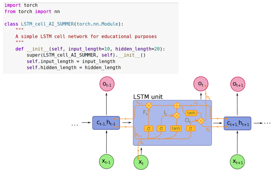
Finally, of all the images that go around online, I found this interesting one to share at this point, for our visual type co-learners:

Image is borrowed from Wiki

Basically, a single cell receives as input the cell and hidden state from the previous timestep, as well as the input vector from the current timestep.
Each LSTM cell outputs the new cell state and a hidden state, which will be used for processing the next timestep. The output of the cell, if needed for example in the next layer, is its hidden state.

Writing a custom LSTM cell in Pytorch - Simplification of LSTM

Based on our current understanding, let’s see in action what the implementation of an LSTM [5] cell looks like. For this implementation PyTorch [6] was used.

Throughout the years, a simpler version of the original LSTM stood the test of time. To this end, modern deep learning frameworks use a slightly simpler version of the LSTM. Actually, they disregard ${c}_{t-1}$ from Equation (1) and (2). And we will do the same. This results in a less complex model that is easier to optimize. Thus, we will implement the following equations:

i_t = \sigma( W_{xi} x_t + W_{hi} {h}_{t-1} + {b}_i) \quad\quad(1)

{f}_t = \sigma( {W}_{xf} {x}_t + {W}_{hf} {h}_{t-1} + {b}_f) \quad\quad(2)

{c}_t = {f}_t \odot {c}_{t-1} + {i}_t \odot tanh( {W}_{xc} x_t + {W}_{hc} {h}_{t-1} + {b}_c ) \quad\quad(3)

{o}_t = \sigma( {W}_{xo} {x}_t + {W}_{h0} {h}_{t-1} + {W}_{co} {c}_{t} + {b}_o) \quad\quad(4)

{h}_t = {o}_t \odot tanh({c}_t) \quad\quad(5)

Nonetheless, it would be interesting for you to tweak the code based on the original implementation and compare the results in this simple task. The code for the simplified LSTM that Pytorch and Tensorflow are running under the hood is the following:

import torch
from torch import nn

class LSTM_cell_AI_SUMMER(torch.nn.Module):
    """
    A simple LSTM cell network for educational AI-summer purposes
    """
    def __init__(self, input_length=10, hidden_length=20):
        super(LSTM_cell_AI_SUMMER, self).__init__()
        self.input_length = input_length
        self.hidden_length = hidden_length

        # forget gate components
        self.linear_forget_w1 = nn.Linear(self.input_length, self.hidden_length, bias=True)
        self.linear_forget_r1 = nn.Linear(self.hidden_length, self.hidden_length, bias=False)
        self.sigmoid_forget = nn.Sigmoid()

        # input gate components
        self.linear_gate_w2 = nn.Linear(self.input_length, self.hidden_length, bias=True)
        self.linear_gate_r2 = nn.Linear(self.hidden_length, self.hidden_length, bias=False)
        self.sigmoid_gate = nn.Sigmoid()

        # cell memory components
        self.linear_gate_w3 = nn.Linear(self.input_length, self.hidden_length, bias=True)
        self.linear_gate_r3 = nn.Linear(self.hidden_length, self.hidden_length, bias=False)
        self.activation_gate = nn.Tanh()

        # out gate components
        self.linear_gate_w4 = nn.Linear(self.input_length, self.hidden_length, bias=True)
        self.linear_gate_r4 = nn.Linear(self.hidden_length, self.hidden_length, bias=False)
        self.sigmoid_hidden_out = nn.Sigmoid()

        self.activation_final = nn.Tanh()

    def forget(self, x, h):
        x = self.linear_forget_w1(x)
        h = self.linear_forget_r1(h)
        return self.sigmoid_forget(x + h)

    def input_gate(self, x, h):

        # Equation 1. input gate
        x_temp = self.linear_gate_w2(x)
        h_temp = self.linear_gate_r2(h)
        i = self.sigmoid_gate(x_temp + h_temp)
        return i

    def cell_memory_gate(self, i, f, x, h, c_prev):
        x = self.linear_gate_w3(x)
        h = self.linear_gate_r3(h)

        # new information part that will be injected in the new context
        k = self.activation_gate(x + h)
        g = k * i

        # forget old context/cell info
        c = f * c_prev
        # learn new context/cell info
        c_next = g + c
        return c_next

    def out_gate(self, x, h):
        x = self.linear_gate_w4(x)
        h = self.linear_gate_r4(h)
        return self.sigmoid_hidden_out(x + h)

    def forward(self, x, tuple_in ):
        (h, c_prev) = tuple_in
        # Equation 1. input gate
        i = self.input_gate(x, h)

        # Equation 2. forget gate
        f = self.forget(x, h)

        # Equation 3. updating the cell memory
        c_next = self.cell_memory_gate(i, f, x, h,c_prev)

        # Equation 4. calculate the main output gate
        o = self.out_gate(x, h)


        # Equation 5. produce next hidden output
        h_next = o * self.activation_final(c_next)

        return h_next, c_next

Connecting LSTM cells across time and space

Let’s see how LSTM’s [5] are connected in time and space. Let’s start from the time perspective, by considering a single sequence of N timesteps and one cell, as it is easier to understand.

As in the first image, we connect the context vector and the hidden states vector, the so-called unrolling. Similarly, we connect the input sequence in the corresponding timestep, x_3 to unrolled cell 3, etc. The size of the unrolled shared-weight cells corresponds to the input sequence timesteps. When you think in terms of time, keep unfolding in the back of your mind.

Let us now imagine how we can connect the cells in space. Suppose we have 2 cells and a single timestep.

The 2 cells are more or less like a different layer. To understand this, let’s just think that the context vector is encapsulated inside the cell, while the hidden state vector is the output. Therefore, we just need to plug the output hidden state of the first cell as the input vector to the next one like this:

hid_{cell1}^{out}(t)= x_{cell2}^{in}(t)

However, don’t confuse it with the hidden vector of the second cell as it is completely different! Less literally, the hidden output of the state of the previous cell is connected as the input vector to the next. The final output is the last hidden cell! As a side note, please keep in mind that different tasks may require all the hidden layer outputs.

Validation: Learning a sine wave with an LSTM

For this proof of concept, we used the official PyTorch example for testing LSTM cells. The code is licensed to authors’ rights. We created an interactive Google Collab notebook so that you can reproduce our results. Basically, what we did is replace torch.nn.LSTMcell() with our own implementation, as presented in this tutorial. You can play around using our Google colab notebook, but note that the original credits of this example belong to the official PyTorch repo. We slightly modified it to maximize understanding for strictly educational purposes. The task is to predict the values of sine wave sequences. The network will subsequently give some predicted results, shown as dash lines.

Simply we replace:

self.lstm1 = nn.LSTMCell(1, 51)
self.lstm2 = nn.LSTMCell(51, 51)

with our own custom implementation and combine everything together in a notebook:

self.lstm1 = LSTM_cell_AI_SUMMER(1,51)
self.lstm2 = LSTM_cell_AI_SUMMER(51,51)

In this way, we focus on ensuring that the rest of the code works ok and if we encounter a problem it will be from our custom code. Let’s see the results!

Results:

Voila!

We have the first validation that proves what the implementation is correct! Even though it is not a great task, it is important to perform these types of sanity checks when you implement custom layers. In addition, in my humble opinion, it enhances our understanding because we focus on mastering the simple concepts, instead of just diving in complex tasks such as activity recognition.

Bidirectional LSTM and it’s Pytorch documentation

In the approach that we described so far, we process the timesteps starting from t=0 to t=N. However, one natural way to expand on this idea is to process the input sequence from the end towards the start. In other words, we start from the end (t=N) and go backwards (until t=0). The opposite direction processing sequence is processed by a different LSTM, but with the same architecture.

Before you set bidirectional=True in your next project think about the implications. Do you want to learn temporal correlations from the end to the start? Does it provide any meaning in your problem? Can you make any assumption about your data that could help you decide that? Note that, by specifying the LSTM to be bidirectional you double the number of parameters. Finally, the hidden/output vector size is also doubled, since the two outputs of the LSTM with different directions are concatenated. A beautiful illustration is depicted below:

Illustration of bidirectional LSTM, borrowed from Cui et al. 2018

Finally, let’s revisit the documentation arguments of Pytorch [6] for an LSTM model. Layers are the number of cells that we want to put together, as we described. Sometimes, dropout is added between LSTM cells.

input_size – The number of expected features in the input x
hidden_size – The number of features in the hidden state h
num_layers – Number of recurrent layers. E.g., setting num_layers=2 would mean stacking two LSTMs together to form a stacked LSTM, with the second LSTM taking in outputs of the first LSTM and computing the final results. Default: 1
bias – If False, then the layer does not use bias weights b_ih and b_hh. Default: True
batch_first – If True, then the input and output tensors are provided as (batch, seq, feature). Default: False
dropout – If non-zero, introduces a Dropout layer on the outputs of each LSTM layer except the last layer, with dropout probability equal to dropout. Default: 0
bidirectional – If True, becomes a bidirectional LSTM. Default: False

Input to output mappings with recurrent models

To avoid possible confusions regarding recurrent layers, let’s start by taking a look in the following image:

The red boxes represent input-to-hidden states,
The green ones represent hidden to hidden states, and
The blue ones represent hidden to output states.

Source: INSA machine learning course notes

The precise input and output can be really messy and frustrating when implementing such a model since the notion of time is often counterintuitive in deep learning. That is why I would like to state that recurrent models are really flexible in the mapping from input to output sequences. You just have to modify the input to hidden states and the hidden to output states, based on the problem. By definition, LSTM’s can process arbitrary input timesteps. The output can be tuned by designing which outputs of the last hidden to hidden layer are used to compute the desired output.

The theoretical limit of modeling a large dimension: Recurrency VS Convolution

Taking our discussion one step further, you can model any dimension by recurrence or by convolution. Why choose one over the other? The hidden magic word that you look for, is the receptive field. Depending on the problem, you want a particular size of the receptive field. In theory, RNN’s can model an infinite size of dimension, which means that their receptive field is infinite. To this end, we still need RNN’s for really long term dependencies such as spoken language and natural language processing. However, it is under discussion if you can use pre-trained models with recurrent units, which is a substantial disadvantage. On the other hand, convolutional neural networks have a finite receptive field [11]. Still, there are a lot of tricks that you can do to increase it, such as dilated convolutions.

Discussion and conclusion

As a final note, the idea of recurrent neural networks can be generalized in multiple dimensions, as described in Graves et al 2007 [7]. In theory, instead of 1D input unrolling we could have a 2D or in general, N-dimensional unrolling. This work was presented by Alex Graves and it is an amazing concept in my humble opinion. Another interesting approach is applying recency in graph-structured data [8].

In a compact sentence, I would like to say that the magic of RNNs lies in the ability to model efficiently long-term dependencies via contextual information. Given the fact you understood the main principles, you can continue to a beautiful TensorFlow tutorial by Google, that presents a very detailed approach for text generation with RNNs.

For further reading, I would suggest this awesome blog post [10] that provides tips about improving the performance in recurrent layers. Alternatively, you can watch the awesome talk that was recently released from DeepMind:

Nevertheless, if you want a more holistic approach in recurrent networks there is an excellent course from Coursera, which we highly recommend. Having said that, we believe that we provided resources for all the different types of learners. Please refer here [3] for a more detailed analysis on RNN optimization.

To conclude, this article serves as an illustration of multiple concepts of recurrent neural networks. We carefully built upon the ideas, in order to understand sequence models that handle time-varying data. We did our best to bridge the gaps between RNN’s in computer vision. In the next part, we will see under the hood of a GRU cell and analyze them side by side.

Cited as:

@article{adaloglou2020rnn,
    title   = "Recurrent neural networks: building a custom LSTM cell",
    author  = "Adaloglou, Nikolas and Karagiannakos, Sergios ",
    journal = "https://theaisummer.com/",
    year    = "2020",
    url     = "https://theaisummer.com/understanding-lstm"
  }

References

[1][understanding lstm networks](https://colah.github.io/posts/2015-08-Understanding-LSTMs/), Cohan’s blog, 2015

[2][a recipe for training neural networks](http://karpathy.github.io/2019/04/25/recipe/), Andrej Karpathy blog, 2019

[3][pptimizing rnn performance](https://svail.github.io/rnn_perf/), Part I: Investigating performance of GPU BLAS Libraries, Erich Elsen, Baidu Silicon Valley AI Lab

[4] Greff, K., Srivastava, R. K., Koutník, J., Steunebrink, B. R., & Schmidhuber, J. (2016). LSTM: A search space odyssey. IEEE transactions on neural networks and learning systems, 28(10), 2222-2232.

[5] Hochreiter, S., & Schmidhuber, J. (1997). Long short-term memory. Neural computation, 9(8), 1735-1780.

[6] Paszke, A., Gross, S., Massa, F., Lerer, A., Bradbury, J., Chanan, G., ... & Desmaison, A. (2019). PyTorch: An imperative style, high-performance deep learning library. In Advances in Neural Information Processing Systems (pp. 8024-8035).

[7] Graves, A., Fernández, S., & Schmidhuber, J. (2007, September). Multi-dimensional recurrent neural networks. In International conference on artificial neural networks (pp. 549-558). Springer, Berlin, Heidelberg.

[8] Agrawal, R., de Alfaro, L., & Polychronopoulos, V. (2017, March). Learning from graph neighborhoods using lstms. In Workshops at the Thirty-First AAAI Conference on Artificial Intelligence.

[9] Horn, R. A. (1990, May). The Hadamard product. In Proc. Symp. Appl. Math (Vol. 40, pp. 87-169).

[10] Danijar Hafner, Tips for Training Recurrent Neural Networks, 2017

[11] Araujo, A., Norris, W., & Sim, J. (2019). Computing Receptive Fields of Convolutional Neural Networks. Distill, 4(11), e21.

[12] Cui, Z., Ke, R., Pu, Z., & Wang, Y. (2018). Deep bidirectional and unidirectional LSTM recurrent neural network for network-wide traffic speed prediction. arXiv preprint arXiv:1801.02143.

* Disclosure: Please note that some of the links above might be affiliate links, and at no additional cost to you, we will earn a commission if you decide to make a purchase after clicking through.