Recurrent Neural Networks: building GRU cells VS LSTM cells in Pytorch

In the previous post, we thoroughly introduced and inspected all the aspects of the LSTM cell. One may argue that RNN approaches are obsolete and there is no point in studying them. It is true that a more recent category of methods called Transformers [5] has totally nailed the field of natural language processing. However, deep learning never ceases to surprise me, RNN’s included. One day maybe we see a huge comeback. Keep in mind that RNN’s are still the best compared to Transformers choice when:

The sequence length is too long.
The task requires real-time control (robotics) or next timesteps are not available a priori.
There is not an enormous dataset to exploit the transfer learning capabilities of transformers.
The computer vision problem is weakly supervised (action recognition). Yes. RNN along with the Connectionist Temporal Classification (CTC) loss [6] still works pretty well.

Other reasons to understand more on RNN include hybrid models. For instance, I recently came across a model [4] that produces realistic real-valued multi-dimensional medical data series, that combines recurrent neural networks and GANs. So you never know where they may come handy.

In any case, fundamentals are to be mastered. This time, we will review and build the Gated Recurrent Unit (GRU), as a natural compact variation of LSTM. Finally, we will provide multiple comparative insights on which cell to use, based on the problem.

Accompanying notebook code is provided here.

GRU: simplifying the LSTM cell

We have seen how LSTM’s are able to predict sequential data. The problem that arose when LSTM’s where initially introduced was the high number of parameters. Let’s start by saying that the motivation for the proposed LSTM variation called GRU is the simplification, in terms of the number of parameters and the performed operations.

Before we jump in the equations let’s clarify one important fact: the principles of LSTM and GRU cells are common, in terms of modeling long-term sequences. First, we can process an arbitrary number of timesteps, Furthermore, we attempt to wash away redundant information and incorporate a memory component stored in the weights. The memory is introduced in the network by the hidden state vector which is unique for each input sequence, each time starting from a zero element vector for $t=0$ .

Now, let’s see the slightly different math! Again, we will analyze them step by step. I am just presenting them here as a reference point.

For $\textbf{x}_t \in R^{N}$ , where N is the feature length of each timestep, while $\textbf{h}_t,\textbf{h}_{t-1}, \textbf{r}_t,\textbf{z}_t,\textbf{z}_{t-1},\textbf{b} \in R^{H}$ , where H is the hidden state dimension, the GRU equations are the following:

\textbf{r}_t = \sigma( \textbf{W}_{ir} \textbf{x}_t + \textbf{b}_{ir} + \textbf{W}_{hr} \textbf{h}_{t-1} + \textbf{b}_{hr} ) \quad\quad(1)

\textbf{z}_t = \sigma( \textbf{W}_{iz} \textbf{x}_t + \textbf{b}_{iz} + \textbf{W}_{hz} \textbf{h}_{t-1} + \textbf{b}_{hz} ) \quad\quad(2)

\textbf{n}_t = tanh(\textbf{W}_{in} \textbf{x}_t + \textbf{b}_{in} + \textbf{r}_t \odot ( \textbf{W}_{hn} \textbf{h}_{t-1} + \textbf{b}_{hn} ) ) \quad\quad(3)

\textbf{h}_t = (1-\textbf{z}_t ) \odot \textbf{n}_t + \textbf{z}_t \odot \textbf{h}_{t-1} \quad\quad(4)

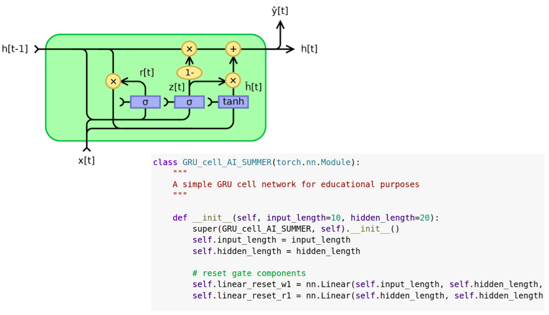
Equation 1: Reset gate

\textbf{r}_t = \sigma( \textbf{W}_{ir} \textbf{x}_t + \textbf{b}_{ir} + \textbf{W}_{hr} \textbf{h}_{t-1} + \textbf{b}_{hr} )

This gate is fairly similar to the forget gate of the LSTM cell. The resulting reset vector r represents the information that will determine what will be removed from the previous hidden time steps. As in the forget gate, we apply the forget operation via element-wise multiplication, denoted by the Hadamard product operator. We calculate the reset vector as a linear combination of the input vector of the current timestep as well as the previous hidden state.

Both operations are calculated with matrix multiplication (nn.Linear in PyTorch). Note that for the first timestep the hidden state is usually a vector filled with zeros. This means that there is no information about the past. Finally, a non-linear activation is applied (i.e. sigmoid). Moreover, by using an activation function (sigmoid) the result lies in the range of (0, 1), which accounts for training stability.

Equation 2: the update gate - the shared update gate vector z

\textbf{z}_t = \sigma( \textbf{W}_{iz} \textbf{x}_t + \textbf{b}_{iz} + \textbf{W}_{hz} \textbf{h}_{t-1} + \textbf{b}_{hz} )

The merging of the input and output gate of the GRU in the so-called update gate happens just here. We calculate another representation of the input vector x and the previous hidden state, but this time with different trainable matrices and biases. The vector z will represent the update vector.

Equation 3: The almost output component

\textbf{n}_t = tanh(\textbf{W}_{in} \textbf{x}_t + \textbf{b}_{in} + \textbf{r}_t \odot ( \textbf{W}_{hn} \textbf{h}_{t-1} + \textbf{b}_{hn} ) )

The vector n consists of two parts; the first one being a linear layer applied to the input, similar to the input gate in an LSTM. The second part consists of the reset vector r and is applied in the previous hidden state. Note that here the forget/reset vector is applied directly in the hidden state, instead of applying it in the intermediate representation of cell vector c of an LSTM cell.

Equation 4: the new hidden state

\textbf{h}_t = (1-\textbf{z}_t ) \odot \textbf{n}_t + \textbf{z}_t \odot \textbf{h}_{t-1}

First of all, in the depicted equation note that 1 is basically a vector of ones. Since the values of z lie in the range (0,1), 1-z also belongs in the same range. However, the elements of the vector z have a complementary value. It is obvious that element-wise operations are applied to z and (1-z).

Sometimes we understand things by analyzing the extreme cases. In an extreme scenario, let’s suppose that z is a vector of ones. What does that mean?

Simply, it means that the input will be ignored, so the next hidden state will be the previous one! In the opposite case that z would be a zero-element vector, it would mean that the previous hidden state is almost ignored. It is important that I use the word almost because the update vector n is affected by the previous hidden state after the reset vector is applied. Still, the recurrence would be almost gone!

Intuitively, the shared vector z balances complementary the influence of the previous hidden state and the update input vector n. Now, it becomes profound why I chose to use the world shared for z. All the above can be illustrated in the following image from Wikipedia:

Source: By Jeblad - Own work, CC BY-SA 4.0, borrowed from Wikipedia

The reason that I am not a big fan of these diagrams, however, is that it may be confusing. This is because they can be interpreted with scalar inputs x and h, which is at least misleading. The second is that it is not clear where the trainable matrices are. Basically, when you think in terms of these diagrams in your RNN journey, try to think that x and h are multiplied by a weight matrix every time they are used. Personally, I prefer to dive into the equations. Fortunately, the maths never lie!

Briefly, the reset gate (r vector) determines how to fuse new inputs with the previous memory, while the update gate defines how much of the previous memory remains.

This is all you need to know so as to understand in-depth how GRU cells work. The way they are connected is exactly the same as LSTM. The hidden output vector will be the input vector to the next GRU cell/layer. A bidirectional could be defined by simultaneously processing the sequence in an inverse manner and concatenating the hidden vectors. In terms of time unrolling in a single cell, the hidden output of the current timestep t becomes the previous timestep in the next one t+1.

LSTM VS GRU cells: Which one to use?

The GRU cells were introduced in 2014 while LSTM cells in 1997, so the trade-offs of GRU are not so thoroughly explored. In many tasks, both architectures yield comparable performance [1]. It is often the case that the tuning of hyperparameters may be more important than choosing the appropriate cell. However, it is good to compare them side by side. Here are the basic 5 discussion points:

It is important to say that both architectures were proposed to tackle the vanishing gradient problem. Both approaches are utilizing a different way of fusing previous timestep information with gates to prevent from vanishing gradients. Nevertheless, the gradient flow in LSTM’s comes from three different paths (gates), so intuitively, you would observe more variability in the gradient descent compared to GRUs.
If you want a more fast and compact model, GRU’s might be the choice, since they have fewer parameters. Thus, in a lot of applications, they can be trained faster. In small-scale datasets with not too big sequences, it is common to opt for GRU cells since with fewer data the expressive power of LSTM may not be exposed. In this perspective, GRU is considered more efficient in terms of simpler structure.
On the other hand, if you have to deal with large datasets, the greater expressive power of LSTMs may lead to superior results. In theory, the LSTM cells should remember longer sequences than GRUs and outperform them in tasks requiring modeling long-range correlations.
Based on the equations, one can observe that a GRU cell has one less gate than an LSTM. Precisely, just a reset and update gates instead of the forget, input, and output gate of LSTM.
Basically, the GRU unit controls the flow of information without having to use a cell memory unit (represented as c in the equations of the LSTM). It exposes the complete memory (unlike LSTM), without any control. So, it is based on the task at hand if this can be beneficial.

To summarize, the answer lies in the data. There is no clear winner to state which one is better. The only way to be sure which one works best on your problem is to train both and analyze their performance. To do so, it is important to structure your deep learning project in a flexible manner. Apart from the cited papers, please note that in order to collect and merge all these pin-out points I advised this and this.) links.

Conclusion

In this article, we provided a review of the GRU unit. We observed it’s distinct characteristics and we even built our own cell that was used to predict sine sequences. Later on, we compared side to side LSTM’s and GRU’s. This time, we will propose for further reading an interesting paper that analyzes GRUs and LSTMs in the context of natural language processing [3] by Yin et al. 2017. As a final RNN resource, we provide this video with multiple visualizations that you may found useful:

Keep in mind that there is no single resource to cover all the aspects of understanding RNN’s, and different individuals learn in a different manner. Our mission is to provide 100% original content in the respect that we focus on the under the hood understanding of RNN’s, rather than deploying their implemented layers in a more fancy application.

Stay tuned for more tutorials.

@article{adaloglou2020rnn,
    title   = "Intuitive understanding of recurrent neural networks",
    author  = "Adaloglou, Nikolas and Karagiannakos, Sergios ",
    journal = "https://theaisummer.com/",
    year    = "2020",
    url     =  "https://theaisummer.com/gru"
  }

References

[1] Greff, K., Srivastava, R. K., Koutník, J., Steunebrink, B. R., & Schmidhuber, J. (2016). LSTM: A search space odyssey. IEEE transactions on neural networks and learning systems, 28(10), 2222-2232.

[2] Chung, J., Gulcehre, C., Cho, K., & Bengio, Y. (2014). Empirical evaluation of gated recurrent neural networks on sequence modeling. arXiv preprint arXiv:1412.3555.

[3] Yin, W., Kann, K., Yu, M., & Schütze, H. (2017). Comparative study of cnn and rnn for natural language processing. arXiv preprint arXiv:1702.01923.

[4] Esteban, C., Hyland, S. L., & Rätsch, G. (2017). Real-valued (medical) time series generation with recurrent conditional gans. arXiv preprint arXiv:1706.02633.

[5] Vaswani, A., Shazeer, N., Parmar, N., Uszkoreit, J., Jones, L., Gomez, A. N., ... & Polosukhin, I. (2017). Attention is all you need. In Advances in neural information processing systems (pp. 5998-6008).

[6] Hannun, "Sequence Modeling with CTC", Distill, 2017.

* Disclosure: Please note that some of the links above might be affiliate links, and at no additional cost to you, we will earn a commission if you decide to make a purchase after clicking through.