Speech Recognition: a review of the different deep learning approaches

Humans communicate preferably through speech using the same language. Speech recognition can be defined as the ability to understand the spoken words of the person speaking.

Automatic speech recognition (ASR) refers to the task of recognizing human speech and translating it into text. This research field has gained a lot of focus over the last decades. It is an important research area for human-to-machine communication. Early methods focused on manual feature extraction and conventional techniques such as Gaussian Mixture Models (GMM), the Dynamic Time Warping (DTW) algorithm and Hidden Markov Models (HMM).

More recently, neural networks such as recurrent neural networks (RNNs), convolutional neural networks (CNNs) and in the last years Transformers, have been applied on ASR and have achieved great performance.

How to formulate Automatic Speech Recognition (ASR)?

The overall flow of ASR can be represented as shown below:

Overview of an ASR system

The main goal of an ASR system is to transform an audio input signal $\mathbf{x} = (x_1, x_2, \dots x_T)$ with a specific length $T$ into a sequence of words or characters (i.e., labels) $\mathbf{y} = ( y_1, y_2, \dots, y_N$ ), $y_{n}\in \mathbf{V}$ , where $\mathbf{V}$ is the vocabulary. The labels might be character-level labels (i.e., letters) or word-level labels (i.e., words).

The most probable output sequence is given by:

\mathbf{\hat{y}} = \argmax_{\mathbf{y} \in \mathbf{V}}~ p(\mathbf{y}|\mathbf{x})

A typical ASR system has the following processing steps:

Pre-processing
Feature extraction
Classification
Language modeling.

The pre-processing step aims to improve the audio signal by reducing the signal-to-noise ratio, reducing the noise, and filtering the signal.

In general, the features that are used for ASR, are extracted with a specific number of values or coefficients, which are generated by applying various methods on the input. This step must be robust, concerning various quality factors, such as noise or the echo effect.

The majority of the ASR methods adopt the following feature extraction techniques:

Mel-frequency cepstral coefficients (MFCCs)
Discrete Wavelet Transform (DWT).

The classification model aims to find the spoken text which is contained on the input signal. It takes the extracted features from the pre-processing step and generates the output text.

The language model (LM) is an important module as it captures the grammatical rules or the semantic information of a language. Language models are important in order to recognize the output token from the classification model as well as to make corrections on the output text.

Datasets for ASR

Various databases with text from audiobooks, conversations, and talks have been recorded.

The CallHome English, Spanish and German databases ( Post et al.¹) contain conversational data with a high number of words, which are not in the vocabulary. They are challenging databases with foreign words and telephone channel distortion. The English CallHome database has 120 spontaneous English telephone conversations between native English people. The training set has 80 conversations of about 15 hours of speech, while the test and development sets contain 20 conversations, where each set has 1.8 hours of audio files.

Moreover, the CallHome Spanish consists of 120 telephone conversations respectively between native speakers. The training part has 16 hours of speech and its test set has 20 conversations with 2 hours of speech. Finally, the CallHome German consists of 100 telephone conversations between native German speakers with 15 hours of speech in the training set and 3.7 hours of speech in the test set.

TIMIT² is a large dataset with broadband recordings from American English, where each speaker reads 10 grammatically rich sentences. TIMIT contains audio signals, which have been time-aligned, corrected and can be used for character or word recognition. The audio files are encoded in 16 bits. The training set contains a large number of audios from 462 speakers in total, while the validation set has audios from 50 speakers and the test set audios from 24 speakers.

Feature extraction for ASR

Mel-frequency Cepstral coefficients is the most common method for extracting speech features. The human ear is a nonlinear system concerning how it perceives the audio signal. In order to cope with the change in frequency, the Mel-scale was developed to make a linear model of the human auditory system. Only frequencies in the range of [0,1] kHz can be transformed to the Mel-scale, while the remaining frequencies are considered to be logarithmic. The mel-scale frequency is computed as:

f_{mel} = \frac{1000}{\log(2)} [1+ \frac{f_{Hz}}{1000}]

where $f_{Hz}$ is the frequency of the original signal.

The MFCC feature extraction technique basically includes the following steps:

Window the signal
Apply Discrete Fourier Transform
Logarithm of the magnitude
Convert to a Mel scale
Apply inverse discrete cosine transform (DCT)

Deep Neural Networks for ASR

In the deep learning era, neural networks have shown significant improvement in the speech recognition task. Various methods have been applied such as convolutional neural networks (CNNs), recurrent neural networks (RNNs), while recently Transformer networks have achieved great performance.

Recurrent Neural Networks

RNNs perform computations on the time sequence since their current hidden state

is dependent on all the previous hidden states. More specifically, they are designed to model time-series signals as well as capture long-term and short-term dependencies between different time-steps of the input.

Concerning speech recognition applications, the input signal $\mathbf{x} = (x_1, x_2, \dots x_T)$ is passed through the RNN to compute the hidden sequences $\mathbf{h} = (h_1, h_2, \dots h_N)$ and the output sequences $\mathbf{y} = (y_1, y_2, \dots y_N)$ , respectively. One major drawback of the simple form of RNNs is that it generates the next output based only on the previous context.

Bidirectional RNN

RNNs compute the sequence of hidden vectors $\mathbf{h}$ as:

\begin{aligned} h_t = H~(W_{xh}x_t + W_{hh}h_{t-1} + b_{h})\\ y_t = W_{hy}h_t + b_{y}, \end{aligned}

where $\mathbf{W}$ are the weights, $\mathbf{b}$ are the bias vectors and $H$ is the nonlinear function.

RNNs limitations and solutions

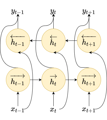
However, in speech recognition, usually the information of the future context is equally significant as the past context (Graves et al.³). That’s why instead of using a unidirectional RNN, bidirectional RNNs (BiRNNs) are commonly selected in order to address this shortcoming. BiRNNs process the input vectors in both directions i.e., forward and backward, and keep the hidden state vectors for each direction as shown in the above figure.

Neural networks, both feed-forward and recurrent, can be only used for frame-wise classification of the input audio.

This problem can be addressed using:

Hidden Markov Models (HMMs) to get the alignment between the input audio and its transcribed output.
Connectionist Temporal Classification (CTC) loss, which is the most common technique.

CTC is an objective function that computes the alignment between the input speech signal and the output sequence of the words. CTC uses a blank label that represents the silence time-step i.e., the person doesn't speak, or represents the transition between words or phonemes. Given the input $\mathbf{x}$ and the output probability sequence of words or characters $\mathbf{y}$ , the probability of an alignment path $\boldsymbol{\alpha}$ is calculated as:

P(\boldsymbol{\alpha}|\mathbf{x}) = \Pi_{t=1}^{T}P(\alpha_t|\mathbf{x})

where $\alpha_t$ is a single alignment at time-step $t$ .

For a given transcription sequence, there are several possible alignments since labels can be separated from blanks in different ways. For example the alignments $(a,-,b,c,-,-)$ and $(-,-$ , $a,-$ , $b,c)$ , ( $-$ is the blank symbol) both correspond to the character sequence $(a,b,c)$ .

Finally, the total probability of all paths is calculated as:

P(\mathbf{y}|\mathbf{x}) = \sum P(\boldsymbol{\alpha}|\mathbf{x})

CTC aims to maximize the total probability of the correct alignments in order to get the correct output word sequence. One main benefit of CTC is that it doesn't require prior segmentation or alignment of the data. DNNs can be used directly to model the features and achieve great performance in speech recognition tasks.

Decoding

The decoding process is used to generate predictions from a trained model using CTC. There are several decoding algorithms. The most common step is the best-path decoding algorithm, where the max probabilities are used in every time-step. Since the model assumes that the latent symbols are independent given the network outputs in the frame-wise case, the output with the highest probability is obtained at each time-step as:

\mathbf{\hat{y}} = \argmax P(\mathbf{y}|\mathbf{x})

Beam search has also been adopted for CTC decoding. The most likely translation is searched using left-to-right time-steps and a small number $B$ of partial hypotheses is maintained. Each hypothesis is actually a prefix of the output sequence, while at each time-step it is extended in the beam with every possible word in the vocabulary.

RNN-Transducer

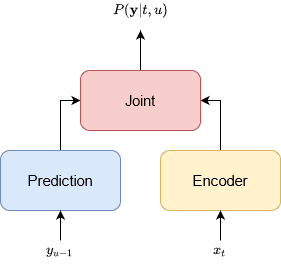
In other works (e.g Rao et al.⁴), an architecture commonly known as RNN-Transducer, has also been employed for ASR. This method combines an RNN with CTC and a separate RNN that predicts the next output given the previous one. It determines a separate probability distribution $P(y_k|t,u)$ for every timestep $t$ of the input and time-step $u$ of the output for the $k$ -th element of the output $\mathbf{y}$ .

An encoder network converts the acoustic feature $x_t$ at time-step $t$ to a representation $he_t = f_{enc}(x_t)$ . Furthermore, a prediction network takes the previous label $y_{u-1}$ and generates a new representation $hp_t = f_{p}(y_{u-1})$ . The joint network is a fully-connected layer that combines the two representations and generates the posterior probability $P(\mathbf{y}|t,u) = f_{joint}(he_t : hp_t)$ . In this way the RNN-Transducer can generate the next symbols or words by using information both from the encoder and the

prediction network based on if the predicted label is a blank or a non-blank label. The inference procedure stops when a blank label is emitted at the last time-step.

RNN Transducer overview

Graves et al.³ tested regular RNNs with CTC and RNN-Transducers in TIMIT² database using different numbers of layers and hidden states.

The feature extraction is performed with a Fourier transform filter-bank method of 40 coefficients that are distributed on a logarithmic mel-scale concatenated with the first and second temporal derivatives.

In the table below, it is shown that RNN-T with 3 layers of 250 hidden states each has the best performance of $17.7\%$ phoneme error rate (PER), while simple RNN-CTC models perform worse with PER $> 18.4\%$ .

RNN performance on TIMIT³

End-to-end ASR with RNN-Transducer (RNN-T)

Rao et al.⁴ proposed an encoder-decoder RNN. The proposed method adopts an encoder network consisting of several blocks of LSTM layers, which are pre-trained with CTC using phonemes, graphemes, and words as output. In addition, 1D-CNN reduces the length $T$ of the time sequence by a factor of 3 using specific kernel strides and sizes.

The decoder network is an RNN-T model trained along with an LSTM language model that also predicts words. The target of the network is the next label in the sequence and is used in the cross-entropy loss to optimize the network. Concerning feature extraction, 80-dimensional mel-scale features are computed every 10 msec and stacked every 30 msec to a single 240-dimensional acoustic feature vector.

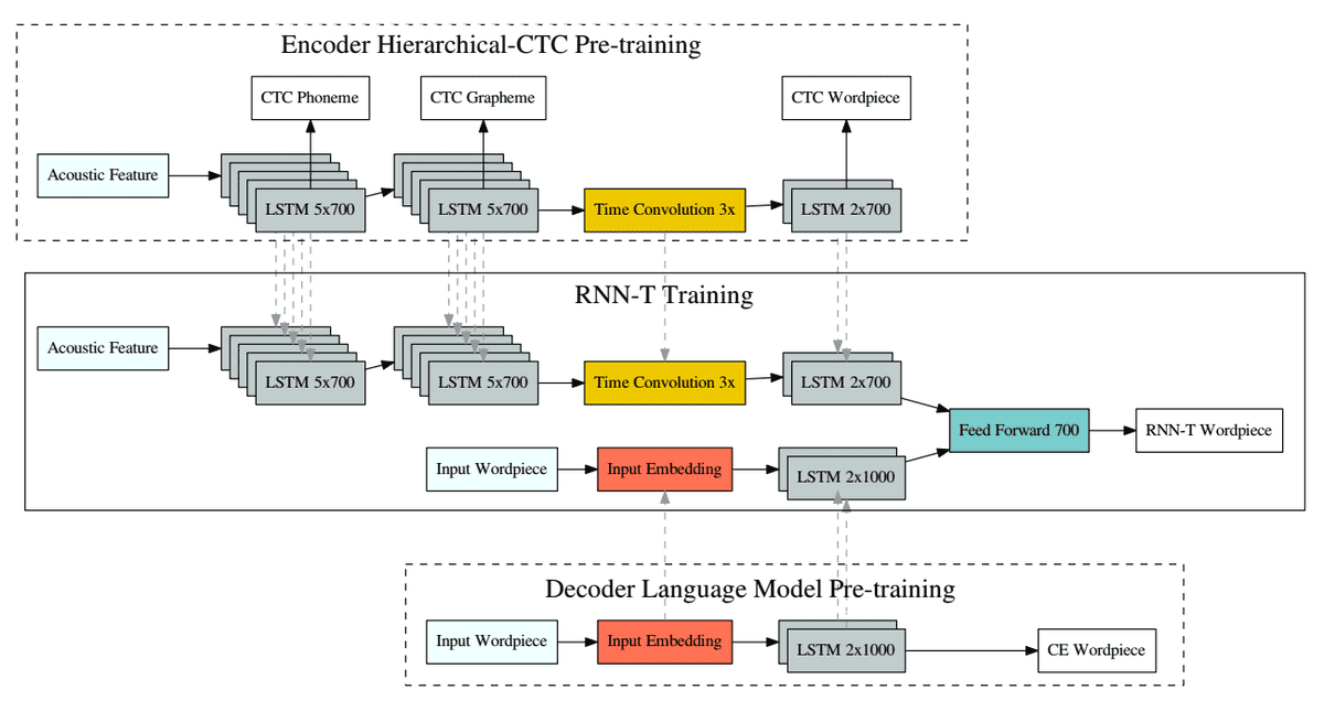RNN-T method⁴

The method is trained on a set of 22 million hand-transcribed audio recordings extracted

from Google US English voice traffic, which corresponds to 18,000 hours of training data. These include voice-search as well as voice-dictation utterances. The language model was pretrained on text sentences obtained from the dataset. The method was tested with different configurations. It achieves $5.2\%$ WER on this large dataset when the encoder contains 12 layers of 700 hidden units and the decoder 2 layers of 1000 hidden units each.

Results from the RNN-T method⁴

Streaming end-to-end speech recognition for mobile devices

RNN-Transducers have also been adopted for real-time speech recognition (He et al.⁵). In this work, the model consists of 8 layers of uni-directional LSTM cells, while a time-reduction layer is used in the encoder to speed up training and inference. Memory caching techniques are also used to avoid redundant computation for identical prediction histories. This saves about $50–60\%$ of the prediction network computations. In addition, different threads are used for the encoder and the prediction network to enable pipe-lining and save a significant amount of time.

The encoder inference procedure is split over two threads corresponding to the components before and after the time-reduction layer, which balances the computation between the

two encoder components and the prediction network, and has a speedup of $28\%$ compared against single-threaded execution. Furthermore, parameters are quantized from 32-bit floating-point precision into 8-bit to reduce memory consumption, both on disk and at run-time, and to optimize the model’s execution in real-time.

The algorithm was trained on a dataset that consists of 35 million English utterances with a size of 27,500 hours. The training utterances are hand-transcribed and are obtained from Google’s voice search and dictation trafﬁc and it was created by artiﬁcially corrupting clean utterances using a room simulator. The reported results are evaluated on 14800 voice search (VS) samples extracted from Google trafﬁc assistant, as well as 15700 voice command samples, denoted as the IME test set. The feature extraction step creates 80-dimensional mel-scale features computed every 25msec. The results are reported in inference speed divided by audio duration (RT90) and WER. The RNN-T model with symmetric quantization achieves WERs of $7.3\%$ on the voice search set and $4.2\%$ on the IME set.

Quantization results⁵

Fast and Accurate Recurrent Neural Network Acoustic Models for ASR

Sak et al.⁶ adopt long-short memory (LSTM) networks for large vocabulary speech recognition. Their method extracts high-dimensional features using mel-filter banks using a sliding window technique. In addition, they incorporate context-dependent states and further improve the performance of the model. The method is evaluated on hand-transcribed audio recordings from real Google voice search traffic. The training set has 3 million utterances with an average duration of 4 seconds. The results are shown in the tables below:

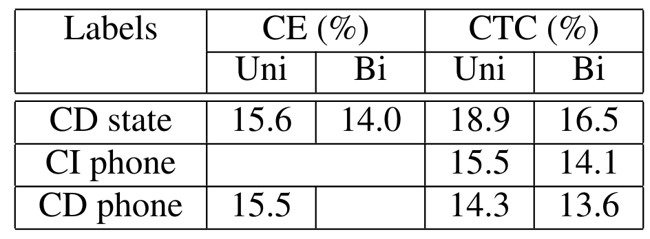Context dependent and independent results⁶

Results with different vocabulary size⁶

Attention-based models

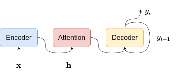
Other works have adopted the attention encoder-decoder structure of the RNN that directly computes the conditional probability of the output sequence given the input sequence without assuming a fixed alignment. The encoder-decoder method uses an attention mechanism, which does not require pre-segment alignment of data. An attention-based model uses a single decoder to produce a distribution over the labels conditioned on the full sequence of previous predictions and the input audio. With attention, it can implicitly learn the soft alignment between input and output sequences, which solves a big problem for speech recognition.

The model can still have a good effect on long input sequences, so it is also possible for such models to handle speech input of various lengths. More specifically, the model computes the output probability density $P(\mathbf{y}|\mathbf{x})$ , where the lengths of the input and output are different. The encoder maps the input to the context vector $\mathbf{c}_i$ for each output $y_i$ . The decoder computes:

P(\mathbf{y}|\mathbf{x}) = \Pi_{i=1}^{I} P(y_i | y_1, \dots, y_{i-1}|\mathbf{c}_i)

conditioned on the $I$ previous outputs and the context $c_i$ .

The posterior probability of symbol $y_i$ is calculated as:

\begin{aligned} P(y_i | y_1, \dots, y_{i-1}|c_i) = g(y_{i-1}, s_i, c_i)\\ s_i = f(y_{i-1}, s_{i-1}, c_i), \end{aligned}

where $s_i$ is the output of the recurrent layer $f$ and $g$ is the softmax function.

The context is obtained from the weighted average of the hidden states of all time-steps as:

\begin{aligned} c_i = \sum_{t=1}^{T} a_{i,t} h_t \\ a_{i,t} = \frac{\mathrm{exp}(e_t)}{\sum_{t=1}^{T}\mathrm{exp}(e_t)}, \end{aligned}

where $a_{i,t} \in [0,1]$ , $\sum_{t=1}^{T} a_{i,t} = 1$ .

The attention mechanism selects the temporal locations over the input sequence that should be used to update the hidden state of the RNN and to predict the next output value. It asserts the attention weights $a_{i,t}$ to compute the relevance scores between the input and the output.

Attention-based recurrent sequence generator

Chorowski et al.⁷, adopts an attention-based recurrent sequence generator (ARSG) that generates the output word sequence from speech features $\mathbf{h} = (h_1, h_2, h_T)$ that can be modelled by any type of encoder. ARSG generates the output $y_i$ by focusing on the relevant features:

\begin{aligned} a_i = \mathrm{attend}(s_{i-1}, a_{i-1}, \mathbf{h})\\ g_i = \sum_{j=1}^{L} a_{i,j}h_j\\ y_i = \mathrm{generate}(s_{i-1}, g_i), \end{aligned}

where $s_i$ is the i-th state of the RNN, $a_i$ are the attention weights.

A new state is generated as:

s_i = recurrency(s_{i-1}, g_i, y_i)

In more detail, the scoring mechanism works as:

e_{i,j} = score~( s_{i-1}, h_i)\\ a_{i,j} = \frac{exp~(e_{i,j}}{\sum_{j=1}^{L}exp~(e_{i,j}}

ARSG is evaluated on the TIMIT dataset and achieves WERs of $15.8\%$ and $17.6\%$ on validation and test sets.

Listen-Attend-Spell (LAS)

In Chan et al⁸ and Chiu et.al⁹ the Listen-Attend-Spell (LAS) method was developed. The encoder (i.e., Listen) takes the input audio $\mathbf{x}$ and generates the representation $\mathbf{h}$ . More specifically, it uses a bidirectional Long Short Term Memory (BLSTM) module with a pyramid structure, where in each layer the time resolution is reduced. The output at the $i$ -th time step, from the $j$ -th layer is computed as:

\begin{aligned} \mathbf{h} = listen~(\mathbf{x})\\ h_i^j = BSLTM~(h_{i-1}^{j}, h_i^{j-1}) \end{aligned}

The decoder (i.e., Attend-Spell) is an attention-based module that attends the representation $\mathbf{h}$ and produces the output probability $P(\mathbf{y}|\mathbf{x})$ . In more detail, an attention-based LSTM transducer produces the next character based on the previous outputs as:

\begin{aligned} c_i = AttentionContext~(s_i, \mathbf{h})\\ s_i = LSTM~(s_{i-1}, y_{i-1}, c_{i-1})\\ P(y_i|\mathbf{x}) = FC~(s_i, c_i), \end{aligned}

where $s_i$ , $c_i$ are the decoder state and the context vector, respectively.

LAS was evaluated on 3 million Google voice search utterances with 2000 hours of speech, where 10 hours of utterances were randomly selected for validation. Data augmentation was also performed on the training dataset using a room simulator noise as well as by adding other types of noise and reverberations. It was able to achieve great recognition rates with WERs of $10.3\%$ and $12,0\%$ on clean and noisy environments, respectively.

Overview of LAS method

End-to-end Speech Recognition with Word-based RNN Language Models and Attention

Hori et al.¹⁰, adopt a joint decoder using CTC, attention decoder, and an RNN language model. A CNN encoder network takes the input audio $\mathbf{x}$ and outputs the hidden sequence $\mathbf{h}$ that is shared between the decoder modules. The decoder network iteratively predicts the 0 label sequence $\mathbf{c}$ based on the hidden sequence. The joint decoder utilizes both CTC, attention and the language model to enforce better alignments between the input and the output and find a better output sequence. The network is trained to maximize the following joint function:

L = \lambda~\mathrm{log} ~p_{CTC} (\mathbf{c}| \mathbf{x}) + (1-\lambda)~ \mathrm{log}~ p_{Att} (\mathbf{c}| \mathbf{x})

During inference, to find the most probable word sequence $\hat{\mathbf{c}}$ , the decoder finds the most probable words as:

\hat{\mathbf{c}} = \mathrm{argmax}~[~p_{CTC} (\mathbf{c}| \mathbf{x}) + (1-\lambda)~ \mathrm{log}~ p_{Att} (\mathbf{c}| \mathbf{x}) + \gamma ~ \mathrm{log} p_{LM}(\mathbf{c})]

where the language model probability is also used. 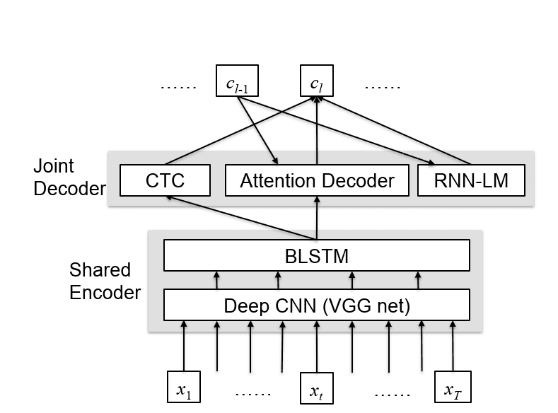Joint decoder

The method is evaluated on Wall Street Journal (WSJ) and LibriSpeech datasets.

WSJ¹¹ is a well-known English clean speech database including approximately 80 hours.

LibriSpeech is a large data set of reading speech from audiobooks and contains 1000 hours of audio and transcriptions¹². The experimental results of the proposed method on WSJ and Librispeech are shown in the following table, respectively.

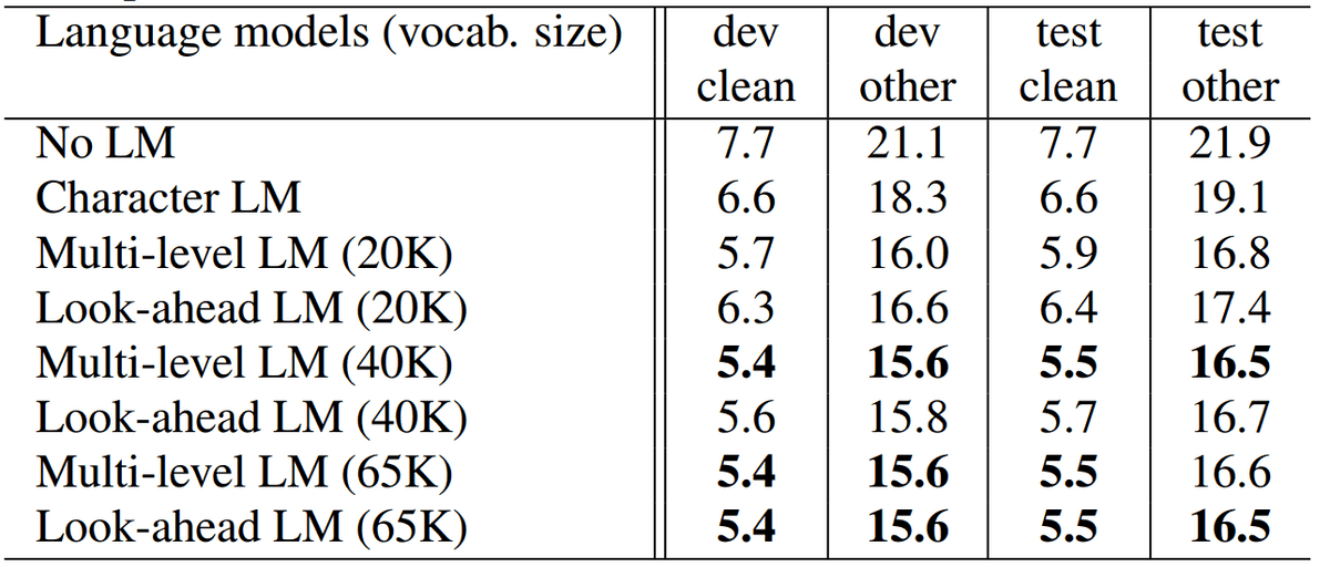Evaluation on the LibriSpeech dataset

Evaluation on the WSJ dataset

Convolutional Models

Convolutional neural networks were initially implemented for computer vision (CV) tasks. In recent years, CNNs have also been widely applied in the field of natural language processing (NLP), due to their good generation, and discrimination capability.

A very typical CNN architecture is formed of several convolutional and pooling layers with fully connected layers for classification. A convolutional layer is composed by kernels that are convolved with the input. A convolutional kernel divides the input signal into smaller

parts namely the receptive field of the kernel. Furthermore, the convolution operation is performed by multiplying the kernel with the corresponding parts of the input that are into the receptive field. Convolutional methods can be grouped into 1-dimensional and 2-dimensional networks, respectively.

2D-CNNs construct 2D feature maps from the acoustic signal. Similar to images, they organize acoustic features i.e., MFCC features, in a 2-dimensional feature map, where one axis represents the frequency domain and the other represents the time domain. In contrast, 1D-CNNs accept acoustic features directly as input.

In 1D-CNN for speech recognition, every input feature map $X=(X_1,\dots, X_I)$ is connected to many feature maps $O = (O_1, \dots, O_J)$ . The convolution operation can be written as:

O_j = \sigma(\sum_{i=1}^{I}X_i w_{i,j} ), ~ j\in[1,J]

where $\mathbf{w}$ is the local weight.

In 1D-CNNs: $\mathbf{w}$ , $\mathbf{O}$ are vectors
In 2D-CNNs they are matrices.

Abdel et al.¹³ were the first that applied CNNs to speech recognition. Their method adopts two types of convolutional layers. The first one adopts full weight sharing (FWS), where weights are shared across. This technique is common in CNNs for image recognition since the same characteristics may appear at any location in an image. However, in speech recognition, the signal varies across different frequencies and has distinct feature patterns in different ﬁlters. To tackle this, limited weight sharing (LWS) is used, where only the convolution filters that are attached to the same pooling filters share the same weights.

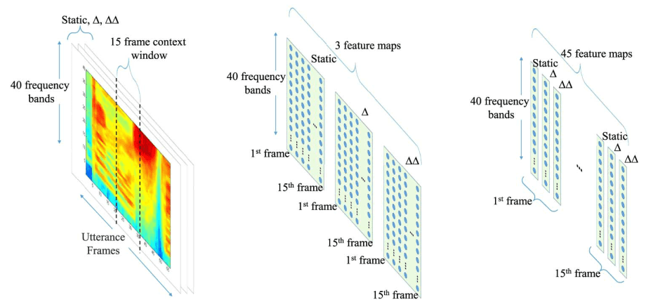Illustration of 2D-CNN feature map for speech recognition¹³

The speech input was analyzed with a 25-ms Hamming window with a fixed 10-ms frame rate. More specifically, feature vectors are generated by Fourier-transform-based filter-bank analysis, which includes40 log energy coefficients distributed on a mel scale, along with

their first and second temporal derivatives. All speech data were normalized so that each vector dimension has a zero mean and unit variance.

The building block of their CNN architecture has convolutions and pooling layers. The input features are organized as several feature maps. The size (resolution) of feature maps gets smaller at upper layers as more convolution and pooling operations are applied as shown in the figure below. Usually, one or more fully connected hidden layers are added

on top of the final CNN layer to combine the features across all frequency bands before feeding to the output layer. They made a comprehensive study with different CNN configurations and achieved great results on TIMIT, which are shown in the below table. Their best model adopts only LWS layers and achieves a WER of $20.23\%$ .

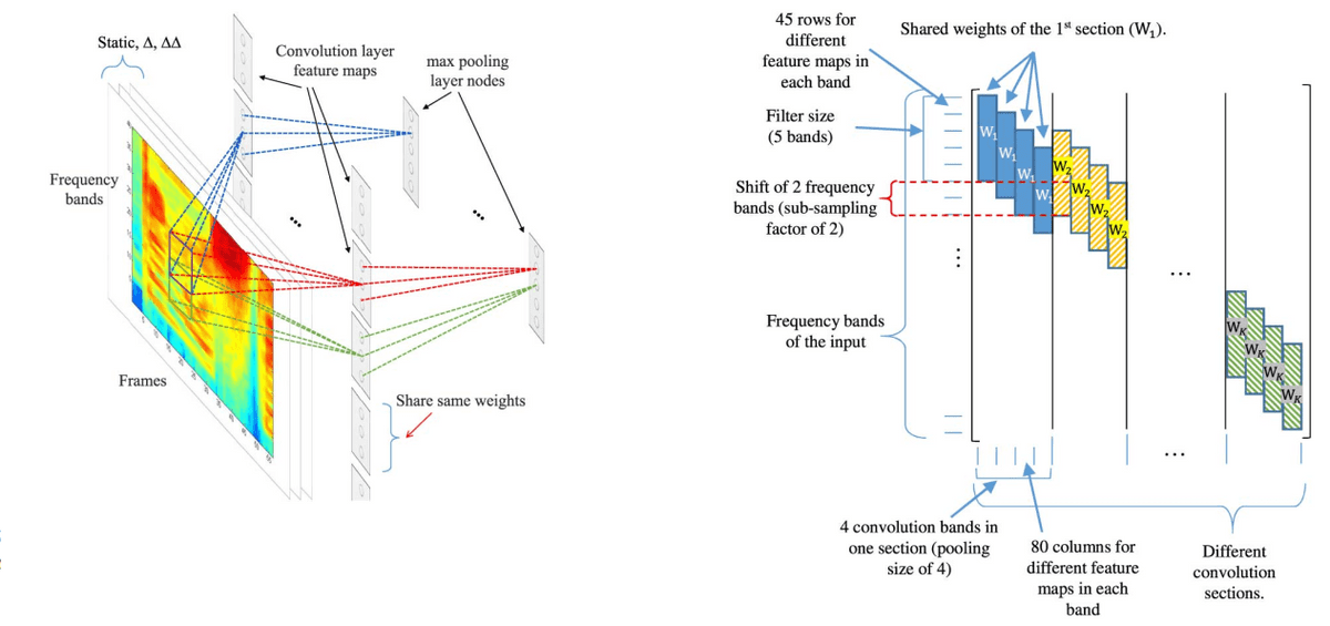Illustration of CNN method¹³

Results of CNN method¹³

Residual CNN

Wang et al.¹⁴ adopted residual 2D-CNN (RCNN) with CTC loss for speech recognition. The residual block uses direct connections between the previous and the next layer as follows:

\mathbf{x}_{i+1} = f~(\mathbf{x}_{i}, \mathbf{W}) + \mathbf{x}_{i}

where $f$ is a nonlinear function. This helps the network to converge faster without the use of extra parameters. The proposed architecture is depicted in the figure below. The Residual CNN-CTC method adopts 4 groups of residual blocks with small $3 \times 3$ ﬁlters. Each Residual group has $N$ number of convolutional blocks with 2 layers. Each residual group also has different strides to reduce the computational cost and model temporal dependencies with different contexts. Batch normalization and ReLU activation are applied on each layer.

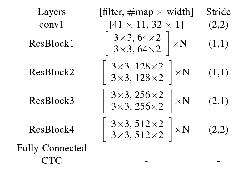Illustration of residual CNN architecture¹⁴

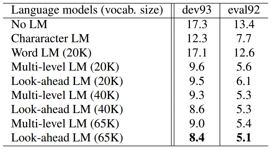
The RCNN is evaluated on WSJ with the standard configuration (si284 set

for training, eval92 set for validation, and dev93 set for testing). Furthermore, it is evaluated on the Tencent Chat data set that contains about 1400 hours of speech data for training and an independent 2000 sentences for test. The experimental results demonstrate the effectiveness of residual convolutional neural networks. RCNN can achieve WERs of $4.29\%/7.65\%$ on validation and test sets of WSJ and $13.33\%$ on the Tencent Chat dataset.

Jasper

Li et al.¹⁵ implemented a residual 1D-CNN with dense and residual blocks as shown below. The network extracts mel-filter-bank features and uses residual blocks that contain batch normalization and dropout layers for faster convergence and better generalization. The input is constructed from mel-filter-bank features obtained using 20 msec windows with a 10 msec overlapping. The network has been tested with different types of normalization and activation functions, while each block is optimized to fit on a single GPU kernel for faster inference. Jasper is evaluated on LibriSpeech with different settings of configuration. The best model has 10 blocks of 4 layers and BatchNorm + ReLU and achieves validation WERs of $6.15\%$ and $17.38\%$ on clean and noisy sets, respectively.

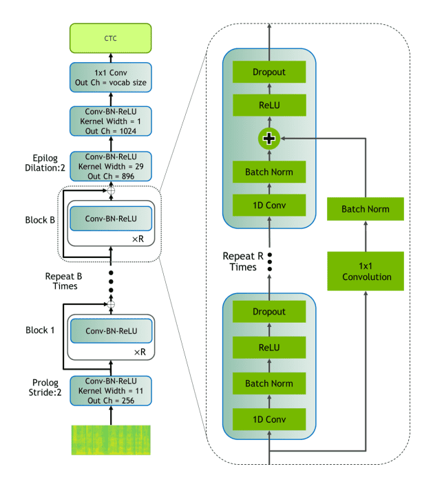Illustration of Jasper¹⁵

Fully Convolutional Network

Zeghidour et al.¹⁶ implement a fully convolutional network (FCN) with 3 main modules. The convolutional front-end is a CNN with low pass filters, convolutional filters similar to filter-banks, and algorithmic function to extract features. The second module is a convolutional acoustic model with several convolutional layers, GELU activation function, dropout, and weight regularization and predicts the letters from the input. Finally, there is a convolutional language model with 14 convolutional residual blocks and bottleneck layers.

This module is used to evaluate the candidate transcriptions of the acoustic model using a beam search decoder. FCN is evaluated on WSJ and LibriSpeech datasets. Their best configuration adopts a trainable convolutional front-end with 80 filters and a convolutional Language model. FCN achieves WERs of $6.8\%$ on the validation set and $3.5\%$ on the test set of WSJ, while on LibriSpeech it achieves validations WERs of $3.08\%/9.94\%$ on clean and noisy sets and testing WERs of $3.26\%/10.47\%$ on clean and noisy sets, respectively.

Illustration of fully convolutional architecture¹⁶

Time-Depth Separable Convolutions (TDS)

Differently from other works, Hannum et al.¹⁷ use time-separable convolutional networks with limited number of parameters and because time-separable CNNs generalize better and are more efficient. The encoder uses 2D depth-wise convolutions along with layer normalization. The encoder outputs two vectors, the keys $\mathbf{k} = k_1, k_2,\dots k_T$ and the values $\mathbf{v} = v_1, v_2,\dots v_T$ from the input sequence $\mathbf{x}$ as:

[\mathbf{k},~ \mathbf{v}] = TSN~(\mathbf{x})

As for the decoder, a simple RNN is used and outputs the next token $y_u$ as:

\begin{aligned} \mathbf{Q}_u = RNN~(y_{u-1}, \mathbf{Q}_{u-1})\\ \mathbf{S}_u = attend (\mathbf{Q}_u, \mathbf{k}, \mathbf{v})\\ y_u = softmax([\mathbf{S}_u , \mathbf{Q}_u]), \end{aligned}

where $\mathbf{S}_u$ is a summary vector and $\mathbf{Q}_u$ is the query vector.

TDS is evaluated on LibriSpeech with different receptive fields and kernel sizes in order to find the best setting for the time-separable convolutional layers. The best option is 11 time-separable blocks, which achieve WERs of $5.04\%$ and $14.46\%$ on dev clean and other sets, respectively.

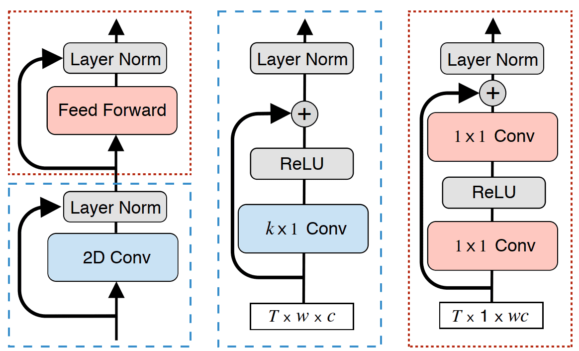2D depth-wise convolutional ASR method¹⁷

ContextNet

ContextNet¹⁸ is a fully convolutional network that feeds global context information into the layers with squeeze-and-excitation modules. The CNN has $K$ layers and generates the features as:

\mathbf{h} = C_K~(C_{K-1}~(\dots (~C_1(\mathbf{x})))),

where $C$ is a convolutional block followed by batch normalization and activation functions. Furthermore, the squeeze-and-excitation block generates a global channel-wise weight $\theta$ with a global average pooling layer, which is multiplied by the input $\mathbf{x}$ as:

\begin{aligned} \mathbf{\bar{x}} = \frac{1}{T}\sum_{t=0}^{T} x_t \\ \theta = \mathrm{fc}~(\mathbf{\bar{x}})\\ SE(\mathbf{x}) = \theta * \mathbf{x} \end{aligned}

ContextNet is validated on LibriSpeech with 3 different conﬁgurations of ContextNet, with or without a language model. The 3 configurations are ContextNet(Small), ContextNet(Medium), and ContextNet(Large), which contain different numbers of layers and filters.

Results on LibriSpeech with 3 different conﬁgurations of ContextNet, with or without language model

Transformers

Recently, with the introduction of Transformer networks¹⁹, machine translation and speech recognition have seen significant improvements. Transformer models that are designed for speech recognition are usually based on the encoder-decoder architecture similar to seq2seq models. In more detail, they are based on the self-attention mechanism instead of recurrence that is adopted by RNNs. The self-attention can attend to different positions of a sequence and extract meaningful representations. The self-attention mechanism takes three inputs, queries, values, and keys.

Let us denote the queries as $\mathbf{Q}\in\mathrm{R^{t_q\times d_q}}$ , the values $\mathbf{V}\in\mathrm{R^{t_v\times d_v}}$ and the keys $\mathbf{K}\in\mathrm{R^{t_k\times d_k}}$ , where $t_{*}$ are the corresponding dimensions. The outputs of self-attention is calculated as:

\mathrm{Attention}(\mathbf{Q},\mathbf{K},\mathbf{V}) = \mathrm{softmax}(\frac{\mathbf{Q}\mathbf{K}^T}{\sqrt{d_k}})\mathbf{V},

where $\frac{1}{\sqrt{d_k}}$ is a scaling factor. However, Transformer adopts the Multi-head attention, which calculates the self-attention $h$ times, one for each head $i$ . In this way, each attention module focuses on different parts and learns different representations. Moreover, the multi-head attention is computed as:

\begin{aligned} \mathrm{ MHA}(\mathbf{Q},\mathbf{K},\mathbf{V}) = \mathrm{concat}(h_1, h_2, \dots h_h)\mathbf{W}^0\\ h_i = \mathrm{Attention}(\mathbf{Q}\mathbf{W}_i^Q,\mathbf{K}\mathbf{W}_i^K,\mathbf{V}\mathbf{W}_i^V), \end{aligned}

where $\mathbf{W}_i^Q\in \mathrm{R}^{d_{model}\times d_q}$ , $\mathbf{W}_i^K\in\mathrm{R}^{d_{model}\times d_k}$ , $\mathbf{W}_i^V\in\mathrm{R}^{d_{model}\times d_v}$ , $\mathbf{W}^O\in \mathrm{R}^{hd_v\times d_{model}}$ and $d_{model}$ the dimensionality of the Transformer. Finally, a feed-forward network is used that contains two fully connected networks and ReLU activation functions as:

\mathrm{FFN(\mathbf{x})} = \mathrm{ReLU}(\mathbf{x}\mathbf{W}_1+\mathbf{b}_1)\mathbf{W}_2+\mathbf{b}_2,

where $\mathbf{W}_1\in \mathrm{R}^{d_{model}\times d_{ff}}, \mathbf{W}_2\in \mathrm{R}^{ d_{ff}\times d_{model}}$ are the weights and $\mathbf{b}_1\in \mathrm{R}^{d_{ff}}, \mathbf{b}_2\in \mathrm{R}^{d_{model}}$ are the biases. In general, to enable the Transformer to attend relative positions, we adopt a positional encoding which is added to the input. The most common technique is the sinusoidal encoding, described by:

\mathbf{PE}(j,i) = \left\{ \begin{array}{ll} { sin(j/10000^{2i/d_{model}}) } {0 \leq i <d_{model}/2} \\ {cos(j/10000^{2i/d_{model}}) } {d_{model}/2 \geq i < d_{model}} \end{array} \right.

where $j,i$ represents the position in the sequence and the $i$ -th dimension, respectively. Finally, normalization layers and residual connections are used to speed up training.

Speech-Transformer

The Speech-Transformer²⁹ transforms the speech feature sequence to the corresponding character sequence. The feature sequence which is longer than the output character sequence is constructed from 2-dimensional spectrograms with time and frequency dimensions. More specifically, CNNs are used to exploit the structure locality of spectrograms and mitigate the length mismatch by striding along time.

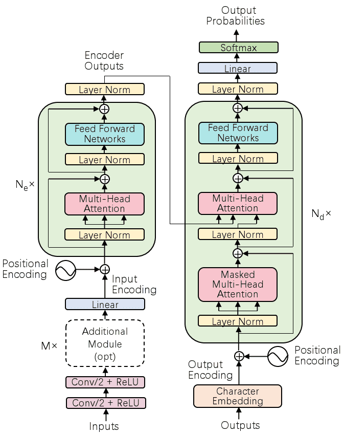Illustration of the Speech Transformer²⁰

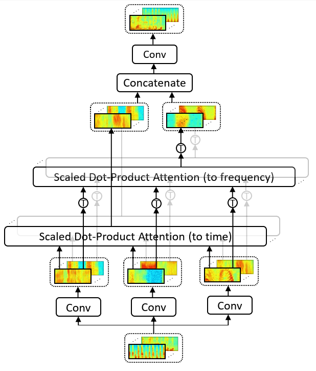Illustration of 2D attention²⁰

In the Speech Transformer, 2D attention is used in order to attend at both the frequency and the time dimensions. The queries, keys, and values are extracted from convolutional neural networks and fed to the two self-attention modules. The Speech Transformer is evaluated on WSJ datasets and achieves competitive recognition results with a WER of $10.9\%$ , while it needs about $80\%$ less training time than conventional RNNs or CNNs.

Transformers with convolutional context

Mohamed et al.²¹ adopt an encoder-decoder model formed by CNNs and a Transformer to learn local relationships and context of the speech signal. For the encoder, 2D convolutional modules with layer normalization and ReLU activation are used. In addition, each 2D convolutional module is formed by $K$ convolutional layers with max-pooling. For the decoder, 1D convolutions are performed over embeddings of the past predicted words.

Transformer-Transducer

Similar to RNN-Transducer, a Transformer-Transducer²² model has also been developed for speech recognition. Compared to RNN-T, this model joint network combines the output of the audio encoder $\mathrm{AE}$ at time-step $t_i$ and the previously predicted label sequence $\mathbf{z}_0^{i-1} = (z_1,..., z_{i-1})$ , which is produced from a feedforward network and a softmax layer, denoted as $\mathrm{LE}$ .

The joint representation is produced as:

J = \mathrm{fc}(\mathrm{AE}(x))(t_i) +\mathrm{fc}(\mathrm{LE}(\mathbf{z}_0^{i-1})),

where $\mathbf{fc}$ is a fully connected layer.

Then, the distribution of the alignment at time-step $t_i$ is computed as:

P(z_i|\mathbf{x}, t_i, \mathbf{z}_0^{i-1}) = \mathrm{softmax}(\mathrm{fc}(J))

Conformer

The Conformer²⁴ is a variant of the original Transformer that combines CNNs and transformers in order to model both local and global speech dependencies by using a more efficient architecture and fewer parameters. The module of the Conformer contains two feedforward layers (FFN), one convolutional layer (CNN), and a multi-head attention module (MHA). The output of the Conformer is computed as:

\begin{aligned} \mathbf{x}_1 = \mathbf{x} + \mathrm{FFN}(\mathbf{x})\\ \mathbf{x}_2 = \mathbf{x}_1 + \mathrm{MHA}(\mathbf{x}_1)\\ \mathbf{x}_3 = \mathbf{x}_2 + \mathrm{CNN}(\mathbf{x}_2)\\ \mathbf{y} = \mathrm{LN}( \mathbf{x}_3 + \mathrm{FFN}(\mathbf{x}_3)) \end{aligned}

Here, the convolutional module adopts efficient pointwise and depthwise convolutions along with layer normalization.

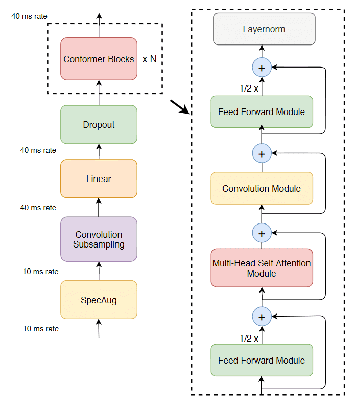Overview of the Conformer method²³

CTC and language models have also been used with Transformer networks²⁴.

Semantic mask for transformer-based ASR

Wang et al.²⁵ utilized a semantic mask of the input speech according to corresponding output tokens in order to generate the next word based on the previous context. A VGG-like convolution layer is used in order to generate short-term dependent features from the input spectrogram, which are then modeled by a Transformer. On the decoder network, the position encoding is replaced by a 1D convolutional layer to extract local features.

Weak-attention suppression or transformer-based ASR

Shi et al.²⁶ propose a weak attention module to suppress non-informative parts of the speech signal such as during silence. The weak attention module sets the attention probabilities smaller than a threshold to zero and normalizes the rest attention probabilities.

The threshold is determined based on the following:

\begin{aligned} \theta_i = m_i -\gamma \delta_i\\ \theta_i = \frac{1}{L}-\gamma \sqrt{\frac{\sum_{j=1}^{L}{(a_{i,j}-\frac{1}{L})}^2}{L-1}} \end{aligned}

Then, softmax is applied again on the new attention probabilities to generate the new attention matrix.

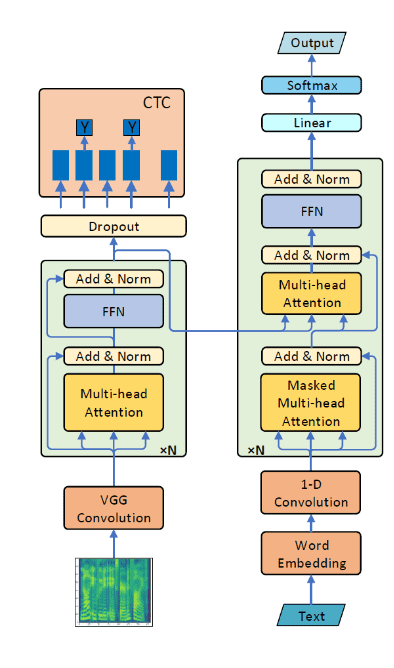Overview of the Semantic Masked Transformer method²⁶

Conclusion

It is evident that deep architectures have already had a significant impact on automatic speech recognition. Convolutional neural networks, recurrent neural networks, and transformers have all been utilized with great success. Today’s SOTA models are all based on some combination of the aforementioned techniques. You can find some benchmarks on the popular datasets on paperswithcode.

If you find this article useful, you might also be interested in a previous one where we review the best speech synthesis methods. And as always, feel free to share it with your friends.

Cite as

@article{papastratis2021speech,
    title   = "Speech Recognition: a review of the different deep learning approaches",
    author  = "Papastratis, Ilias",
    journal = "https://theaisummer.com/",
    year    = "2021",
    howpublished = {https://theaisummer.com/speech-recognition/},
  }

References

Matt Post, Gaurav Kumar, Adam Lopez, Damianos Karakos, Chris Callison-Burch, and Sanjeev Khudanpur, “Improved speech-to-text translation with the Fisher and Callhome Spanish–English speech translation corpus,” inProceedings of the International Workshop on Spoken Language Translation(IWSLT), Heidelberg, Germany, December 2013.↩
John S Garofolo, “Timit acoustic phonetic continuous speech corpus,” Linguistic Data Consortium, 1993, 1993.↩
Alex Graves, Abdel-rahman Mohamed, and Geoffrey Hinton, “Speech recognition with deep recurrent neural networks,” in2013 IEEE international conference on acoustics, speech and signal processing. Ieee, 2013, pp. 6645–6649.↩
Kanishka Rao, Ha ̧sim Sak, and Rohit Prabhavalkar, “Exploring architectures, data, and units for streaming end-to-end speech recognition with rnn-transducer,” in2017 IEEE Automatic Speech Recognition and Understanding Workshop (ASRU), 2017, pp. 193–199.↩
Yanzhang He, Tara N Sainath, Rohit Prabhavalkar, Ian McGraw, Raziel Alvarez, Ding Zhao, David Rybach, Anjuli Kannan, Yonghui Wu, RuomingPang, et al., “Streaming end-to-end speech recognition for mobile devices,”inICASSP 2019-2019 IEEE International Conference on Acoustics, Speech and Signal Processing (ICASSP). IEEE, 2019, pp. 6381–6385.31↩
Ha ̧sim Sak, Andrew Senior, Kanishka Rao, and Françoise Beaufays, “Fast and accurate recurrent neural network acoustic models for speech recognition,”arXiv preprint arXiv:1507.06947, 2015.↩
Jan Chorowski, Dzmitry Bahdanau, Dmitriy Serdyuk, Kyunghyun Cho, and Yoshua Bengio, “Attention-based models for speech recognition,”arXivpreprint arXiv:1506.07503, 2015.↩
William Chan, Navdeep Jaitly, Quoc Le, and Oriol Vinyals, “Listen, attend and spell: A neural network for large vocabulary conversational speech recognition,” in2016 IEEE International Conference on Acoustics, Speech and Signal Processing (ICASSP). IEEE, 2016, pp. 4960–4964.↩
Chung-Cheng Chiu, Tara N Sainath, Yonghui Wu, Rohit Prabhavalkar, Patrick Nguyen, Zhifeng Chen, Anjuli Kannan, Ron J Weiss, Kanishka Rao, Ekaterina Gonina, et al., “State-of-the-art speech recognition with sequence-to-sequence models,” in2018 IEEE International Conference on Acoustics, Speech and Signal Processing (ICASSP). IEEE, 2018, pp. 4774–4778.↩
Takaaki Hori, Jaejin Cho, and Shinji Watanabe, “End-to-end speech recognition with word-based rnn language models,” in2018 IEEE Spoken LanguageTechnology Workshop (SLT), 2018, pp. 389–396.↩
Douglas B Paul and Janet Baker, “The design for the wall street journal-based csr corpus,” in Speech and Natural Language: Proceedings of a Workshop Held at Harriman, New York, February 23-26, 1992, 1992.↩
Vassil Panayotov, Guoguo Chen, Daniel Povey, and Sanjeev Khudanpur, “Librispeech: an asr corpus based on public domain audio books,” in2015IEEE international conference on acoustics, speech and signal processing(ICASSP). IEEE, 2015, pp. 5206–5210.↩
Ossama Abdel-Hamid, Abdel-rahman Mohamed, Hui Jiang, Li Deng, Gerald Penn, and Dong Yu, “Convolutional neural networks for speech recognition,” IEEE/ACM Transactions on audio, speech, and language processing, vol. 22, no. 10, pp. 1533–1545, 2014.↩
Yisen Wang, Xuejiao Deng, Songbai Pu, and Zhiheng Huang, “Residual convolutional ctc networks for automatic speech recognition,”arXiv preprintarXiv:1702.07793, 2017.↩
Jason Li, Vitaly Lavrukhin, Boris Ginsburg, Ryan Leary, Oleksii Kuchaiev, Jonathan M Cohen, Huyen Nguyen, and Ravi Teja Gadde, “Jasper: An end-to-end convolutional neural acoustic model,”arXiv preprintarXiv:1904.03288, 2019.↩
Neil Zeghidour, Qiantong Xu, Vitaliy Liptchinsky, Nicolas Usunier, GabrielSynnaeve, and Ronan Collobert, “Fully convolutional speech recognition,”arXiv e-prints, pp. arXiv–1812, 2018.↩
Awni Hannun, Ann Lee, Qiantong Xu, and Ronan Collobert, “Sequence-to-sequence speech recognition with time-depth separable convolutions,”arXivpreprint arXiv:1904.02619, 2019.↩
Wei Han, Zhengdong Zhang, Yu Zhang, Jiahui Yu, Chung-Cheng Chiu, James Qin, Anmol Gulati, Ruoming Pang, and Yonghui Wu, “Contextnet: Improving convolutional neural networks for automatic speech recognition with global context,”arXiv preprint arXiv:2005.03191, 2020.↩
Ashish Vaswani, Noam Shazeer, Niki Parmar, Jakob Uszkoreit, Llion Jones,Aidan N Gomez, Lukasz Kaiser, and Illia Polosukhin, “Attention is all you need,”arXiv preprint arXiv:1706.03762, 2017.↩
Linhao Dong, Shuang Xu, and Bo Xu, “Speech-transformer: a no-recurrence sequence-to-sequence model for speech recognition,” in2018 IEEE Inter-national Conference on Acoustics, Speech and Signal Processing (ICASSP).IEEE, 2018, pp. 5884–5888.↩
Abdelrahman Mohamed, Dmytro Okhonko, and Luke Zettlemoyer, “Transformers with convolutional context for asr,”arXiv preprintarXiv:1904.11660, 2019.↩
Qian Zhang, Han Lu, Hasim Sak, Anshuman Tripathi, Erik McDermott, Stephen Koo, and Shankar Kumar, “Transformer transducer: A streamable speech recognition model with transformer encoders and rnn-t loss,”inICASSP 2020-2020 IEEE International Conference on Acoustics, Speech and Signal Processing (ICASSP). IEEE, 2020, pp. 7829–7833.↩
Shigeki Karita, Nelson Enrique Yalta Soplin, Shinji Watanabe, Marc Del-croix, Atsunori Ogawa, and Tomohiro Nakatani, “Improving transformer-based end-to-end speech recognition with connectionist temporal classification and language model integration,”Proc. Interspeech 2019, pp. 1408–1412, 2019.↩
Anmol Gulati, James Qin, Chung-Cheng Chiu, Niki Parmar, Yu Zhang, Ji-ahui Yu, Wei Han, Shibo Wang, Zhengdong Zhang, Yonghui Wu, et al., “Conformer: Convolution-augmented transformer for speech recognition,”arXiv preprint arXiv:2005.08100, 2020.↩
Chengyi Wang, Yu Wu, Yujiao Du, Jinyu Li, Shujie Liu, Liang Lu, Shuo Ren, Guoli Ye, Sheng Zhao, and Ming Zhou, “Semantic mask for transformer-based end-to-end speech recognition,”arXiv preprintarXiv:1912.03010, 2019.↩
Yangyang Shi, Yongqiang Wang, Chunyang Wu, Christian Fuegen, FrankZhang, Duc Le, Ching-Feng Yeh, and Michael L Seltzer, “Weak-attention suppression for transformer-based speech recognition,”arXiv preprintarXiv:2005.09137, 2020↩

* Disclosure: Please note that some of the links above might be affiliate links, and at no additional cost to you, we will earn a commission if you decide to make a purchase after clicking through.