Speech synthesis is the task of generating speech from some other modality like text, lip movements, etc. In most applications, text is chosen as the preliminary form because of the rapid advance of natural language systems. A Text To Speech (TTS) system aims to convert natural language into speech.
Over the years there have been many different approaches, with the most prominent being concatenation synthesis and parametric synthesis.
Concatenation synthesis
Concatenation synthesis, as the name suggests, is based on the concatenation of pre-recorded speech segments. The segments can be full sentences, words, syllables, diphones, or even individual phones. They are usually stored in the form of waveforms or spectrograms.
We acquire the segments with the help of a speech recognition system and we then label them based on their acoustic properties (e.g. their fundamental frequency). At run time, the desired sequence is created by determining the best chain of candidate units from the database (unit selection).
Statistical Parametric Synthesis
Parametric synthesis utilizes recorded human voices as well. The difference is that we use a function and a set of parameters to modify the voice. Let’s break that down:
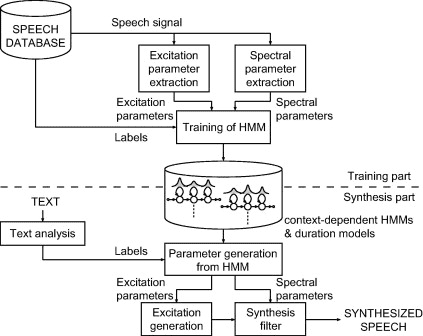 Statistical parametric speech synthesis
In statistical parametric synthesis, we generally have two parts. The training and the synthesis. During training, we extract a set of parameters that characterize the audio sample such as the frequency spectrum (vocal tract), fundamental frequency (voice source), and duration (prosody) of speech. We then try to estimate those parameters using a statistical model. The one that has been proven to provide the best results historically is the Hidden Markov Model (HMM).
During synthesis, HMMs generate a set of parameters from our target text sequence. The parameters are used to synthesize the final speech waveforms.
Advantages of statistical parametric synthesis:
No need to store audio sample in a database
Language independence
Flexibility in voice characteristics
However, in most cases, the quality of the synthesized speech is not ideal. This is where Deep Learning based methods come into play.
But before that, I would like to open a small parenthesis and discuss how we evaluate speech synthesis models.
Speech synthesis evaluation
Mean Opinion Score (MOS) is the most frequently used method to evaluate the quality of the generated speech. MOS has a range from 0 to 5 where real human speech is between 4.5 to 4.8
MOS comes from the telecommunications field and is defined as the arithmetic mean over single ratings performed by human subjects for a given stimulus in a subjective quality evaluation test. This historically means that a group of people sits in a quiet room, listens to the generated sample, and gives it a score. MOS is nothing more than the average of all “people’s opinion”
Today’s benchmarks are performed over different speech synthesis datasets in English, Chinese, and other popular languages. You can find such benchmarks in paperswithcode.com
Speech synthesis with Deep Learning
Before we start analyzing the various architectures, let’s explore how we can mathematically formulate TTS.
Given an input text sequence , the target speech can be derived by:
where is the model’s parameters.
In most models, we first pass the input text to an acoustic feature generator, which produces a set of acoustic features such as the fundamental frequency or spectrogram.
To generate the final speech segment, a Neural vocoder is typically used.
A traditional vocoder is a category of voice codec which encrypts and compresses the audio signal and vice versa. This was traditionally accomplished through digital signal processing techniques. A neural vocoder achieves the encoding/decoding using a neural network.
WaveNet
WaveNet was the first model that successfully modeled the raw waveform of the audio signal instead of the acoustic features. It is able to generate new speech-like waveforms at 16,000 samples per second.
WaveNet in its core is an autoregressive model where each sample depends on the previous ones. Mathematically, this can be expressed as :
In essence, we factorize the joining probability of the waveform as a product of conditional probabilities of the previous time steps.
To build such autoregressive models, the authored used a fully convolutional neural network with dilated convolutions. WaveNet was inspired by PixelCNN and PixelRNN, which are able to generate very complex natural images.
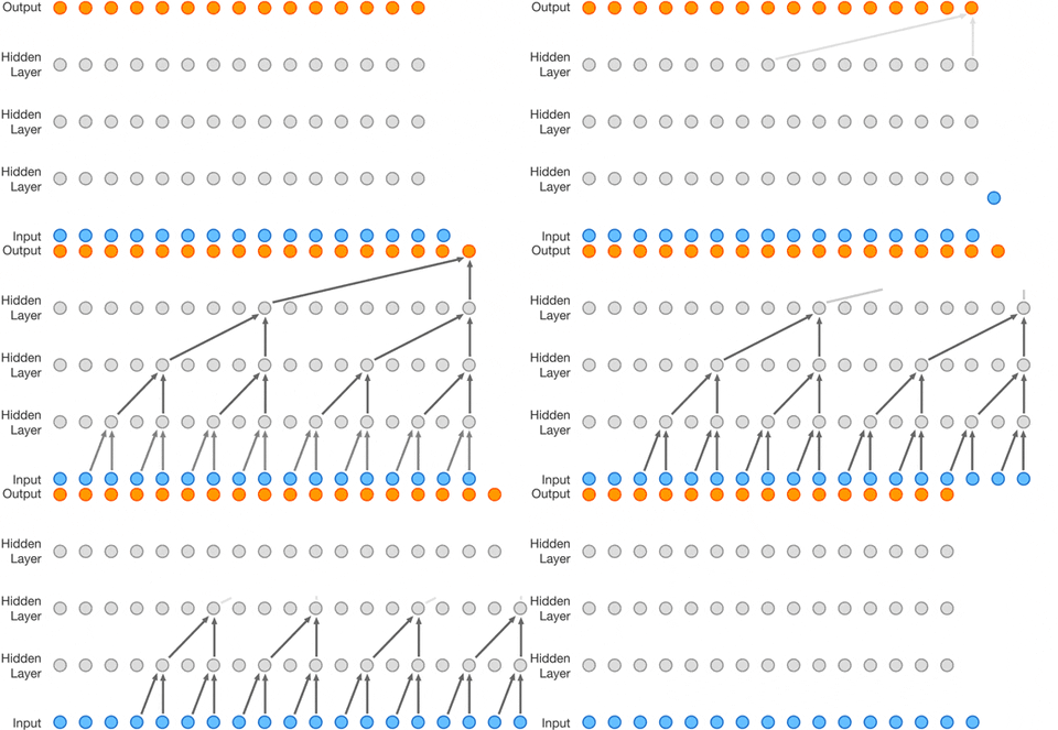 Source:WaveNet: A generative model for raw audio
As we can see in the image above, each convolutional layer has a dilation factor. They used real waveforms recorded from human speakers during training. After training, the final waveform is produced by sampling from the network. How the sampling is performed?
The autoregressive model computes the probability distribution . At each timestep:
We sample a value from the distribution
We feed the value back to the input, and the model generates the new prediction
We continue this procedure one step at a time to generate the entire speech waveform.
This is the main shortcoming of WaveNet. Because we need to perform this for every simple sample, inferences can become very slow and computationally expensive
The first version of WaveNet managed to has a MOS of 4.21 in the English language where for previous state of art models, MOS was between 3.67 and 3.86.
Fast WaveNet
Fast WaveNet managed to reduce the complexity of the original WaveNet from to where is the number of layers in the network. This was achieved by introducing a caching system that stored previous calculations. That way no redundant convolutions were ever be calculated.
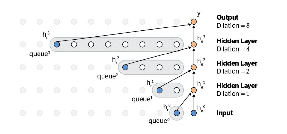 The caching scheme of Fast WaveNet. Source: Fast WaveNet Generation Algorithm
Deep Voice
Deep Voice by Baidu laid the foundation for the later advancements on end-to-end speech synthesis. It consists of 4 different neural networks that together form an end-to-pipeline.
A segmentation model that locates boundaries between phonemes. It is a hybrid CNN and RNN network that is trained to predict the alignment between vocal sounds and the target phonemes using the CTC loss.
A model that converts graphemes to phonemes. A multi-layer encoder-decoder model with GRU cells was chosen for this task.
A model to predict phonemes duration and the fundamental frequencies. Two fully connected layers followed by two unidirectional GRU layers and another fully connected layer, were trained to learn both tasks simultaneously
A model to synthesize the final audio. Here the authors implemented a modified WaveNet. The WaveNet consists of a conditioning network that upsamples linguistic features to the desired frequency, and an autoregressive network, which generates a probability distribution P over discretized audio samples
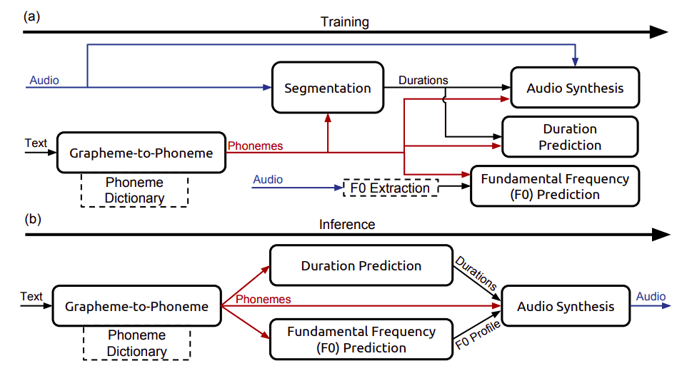 System diagram depicting (a) training procedure and (b) inference procedure of DeepVoice. Source: Deep Voice: Real-time Neural Text-to-Speech
They also managed to achieve real-time inference by constructing highly optimized CPU and GPU kernels to speed up the inference. It received a MOS of 2.67 in US English.
Tacotron
Tacotron was released by Google in 2017 as an end-to-end system. It is basically a sequence to sequence model that follows the familiar encoder-decoder architecture. An attention mechanism was also utilized.
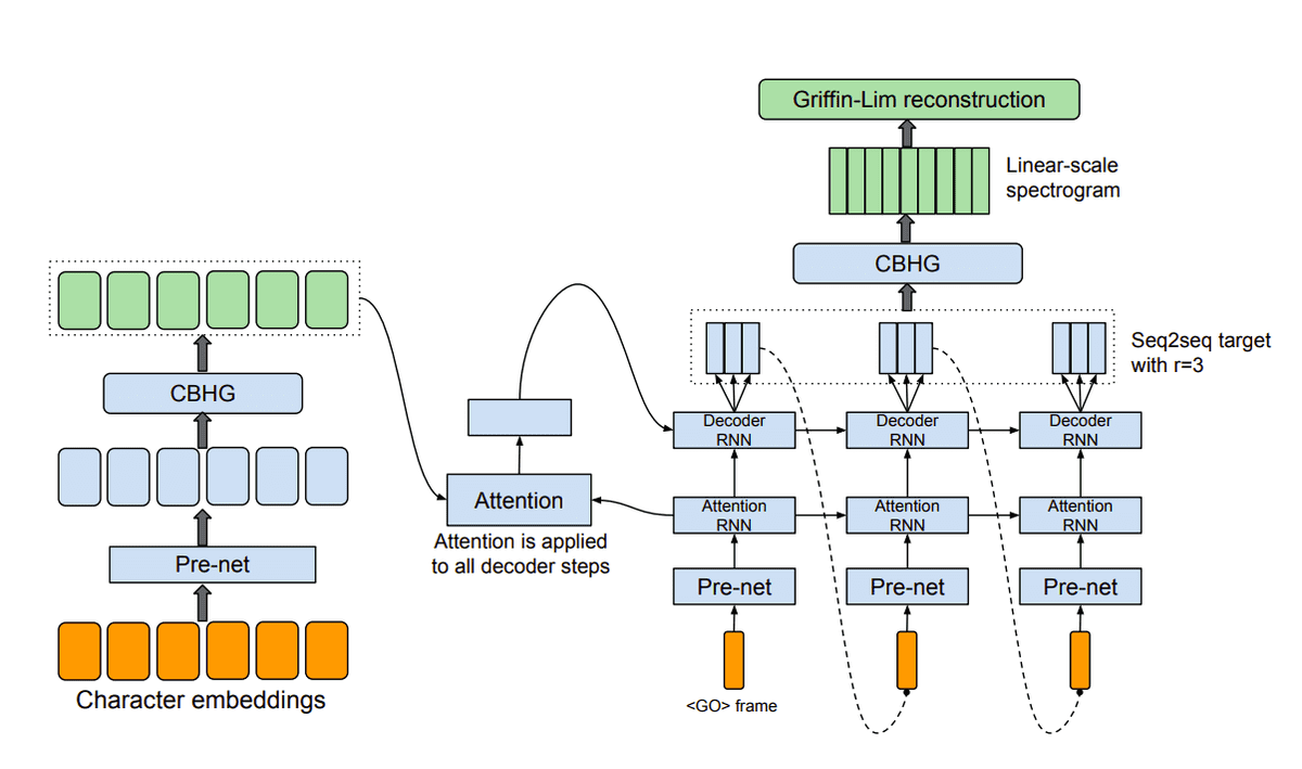 Source: Tacotron: Towards End-to-End Speech Synthesis
Let’s break down the above diagram.
The model takes as input characters and outputs the raw spectrogram of the final speech, which is then converted to waveform.
The CBHG module
You might wonder what is this CBHG. CBHG stands for: 1-D convolution bank + highway network + bidirectional GRU. The CBHG module is used to extract representations from sequences, and it was originally developed for neural machine translation. The below diagram will give you a better understanding:
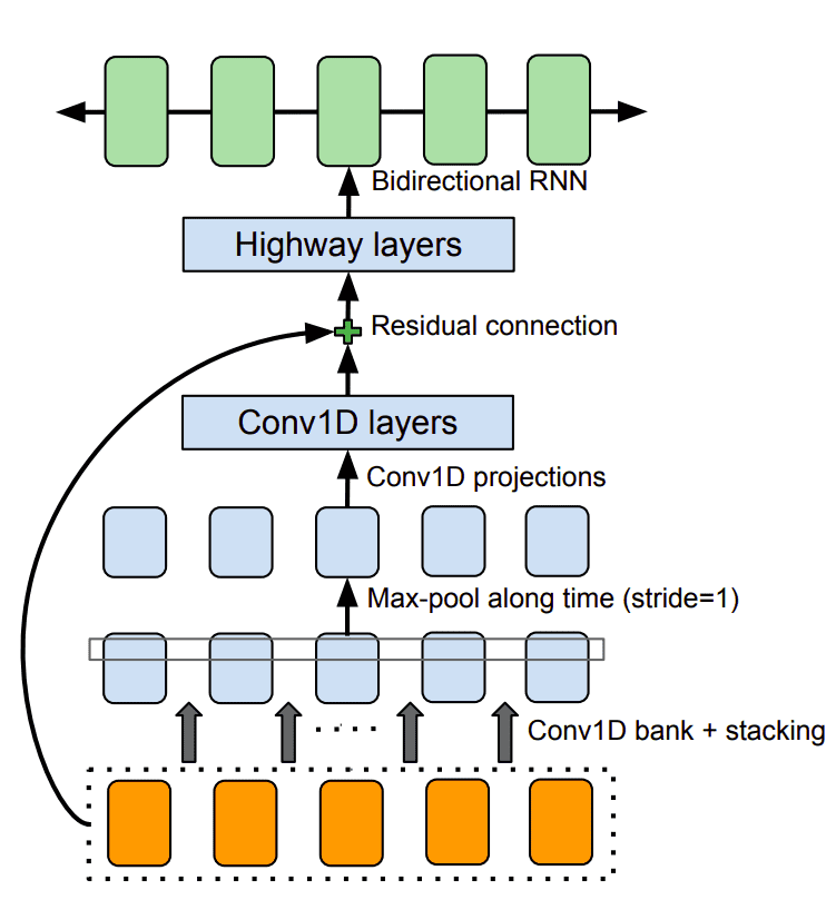 The CBHG module. Source: Tacotron: Towards End-to-End Speech Synthesis
Back to Tacotron. The encoder’s goal is to extract robust sequential representations of text. It receives a character sequence represented as one-hot encoding and through a stack of PreNets and CHBG modules, it outputs the final representation. PreNet is used to describe the non-linear transformations applied to each embedding.
Content-based attention is used to pass the representation to the decoder, where a recurrent layer produces the attention query at each time step. The query is concatenated with the context vector and passed to a stack of GRU cells with residual connections. The output of the decoder is converted to the end waveform with a separate post-processing network, containing a CBHG module.
Tacotron achieved a MOS of 3.82 on an US English evaluation set.
Deep Voice 2
Deep Voice 2 came as an improvement of the original Deep Voice architecture. While the main pipeline was quite similar, each model was created from scratch to enhance its performance. Another big enhancement was the addition of multi-speaker support.
Key points of the architecture:
Separation of the phoneme duration and fundamental frequency models
Speaker embeddings were introduced on each model to achieve multiple-speaker capabilities. The speaker embeddings hold the unique information per speaker and are used to produce recurrent neural network (RNN) initial states, nonlinearity biases, and multiplicative gating factors, used throughout the networks.
Batch normalization and residual connections were applied to the basic models
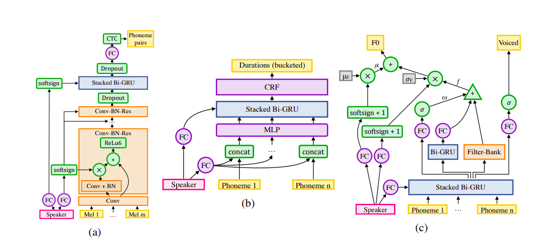 Segmentation, duration and frequency models of DeepVoice 2. Source: Deep Voice 2: Multi-Speaker Neural Text-to-Speech
A surprising fact is that the authors showed, in the same paper, that we can also enhance Tacotron to support multi-speakers using similar techniques. Moreover, they replace Tacotron’s spectrogram-to-waveform Model with their own WaveNet-based neural vocoder and the results were very promising
DeepVoice 2 with an 80-layer WaveNet, as the sound synthesizer model, achieved a MOS of 3.53
Deep Voice 3
Deep Voice 3 is a complete redesign of the previous versions. Here we have a single model instead of four different ones. More specifically, the authors proposed a fully-convolutional character-to-spectrogram architecture which is ideal for parallel computation. As opposed to RNN-based models. They were also experimenting with different waveform synthesis methods with the WaveNet achieving the best results once again.
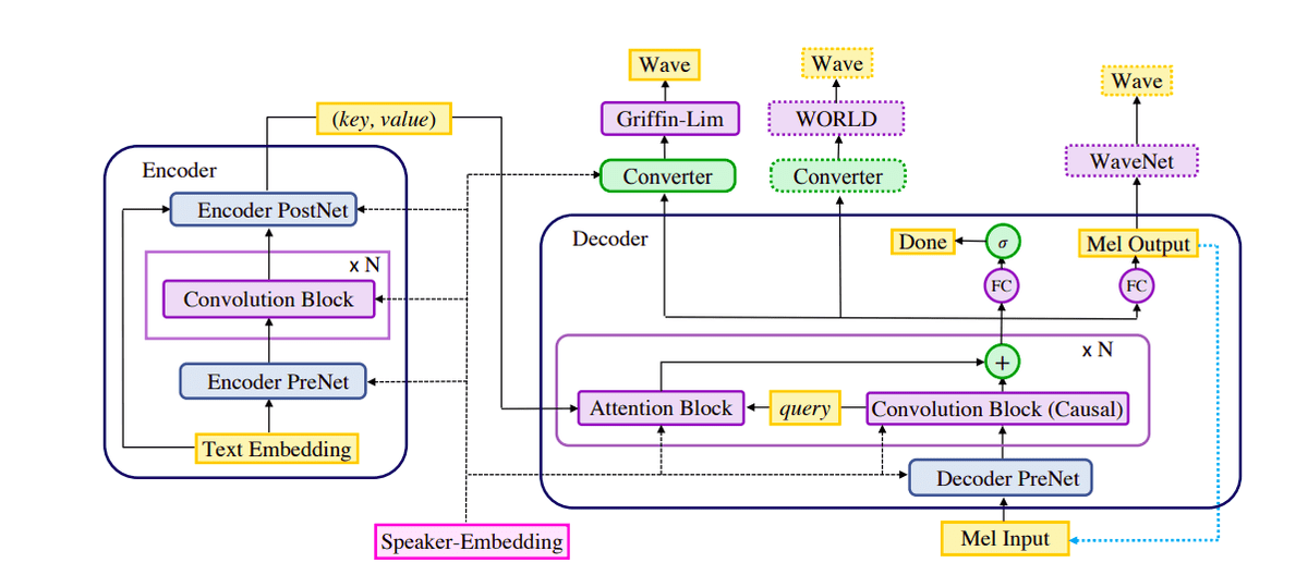 Deep Voice 3: Scaling Text-to-Speech with Convolutional Sequence Learning
As you can see, Deep Voice 3 is an encoder-decoder architecture and is able to produce a variety of textual features(character, phonemes, etc.) to a variety of vocoder parameters.
The encoder is a fully-convolutional neural network that transforms textual features into a compact representation. The decoder is another fully-convolutional network that converts the learned representation into a low-dimensional audio representation. This is achieved using a multi-hop convolutional attention mechanism.
The convolution block comprises 1-D convolutions followed by a GRU cell and a residual connection.
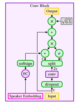 The convolution block of Deep Voice 3. Source: Deep Voice 3: Scaling Text-to-Speech with Convolutional Sequence Learning
The attention mechanism uses a query vector (the hidden states of the decoder) and the per-timestep key vectors from the encoder to compute attention weights. It then outputs a context vector as the weighted average of the value vectors.
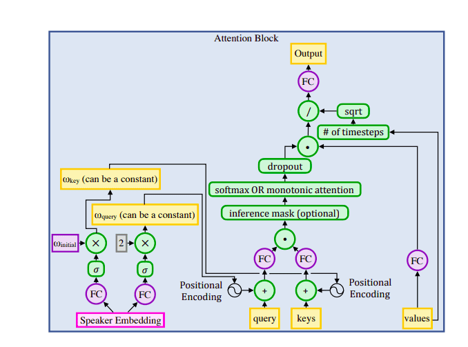 Attention block of Deep Voice 3. Source: Deep Voice 3: Scaling Text-to-Speech with Convolutional Sequence Learning
Deep Voice 3 with WaveNet achieved a MOS of 3.78 at the time of publishing
Parallel WaveNet
Parallel WaveNet aims to solve the complexity and performance issues of the original WaveNet, which relies on sequential generation of the audio, one sample at a time.
They introduced a concept called Probability Density Distillation that tries to marry Inverse autoregressive flows with efficient WaveNet training methods.
Inverse autoregressive flows (IAFs) represent a kind of dual formulation of deep autoregressive modelling, in which sampling can be performed in parallel. IAFs are stochastic generative models whose latent variables are arranged so that all elements of a high dimensional observable sample can be generated in parallel
Let’s break that down and explain it in simple terms:
Because each sample depends on the previous ones, we can’t simple parallelized this process and compute them in parallel. Instead, we start out from simple white noise and apply changes over time until it morphs to the desired output waveform. These changes are applied to the entire signal in a parallel fashion. How?
We use a teacher-student relationship. The teacher is the original Network that holds the ground truth but it is quite slow. The student is the new network that tries to mimic the teacher but in a more efficient way.
According to the authors: “To stress the fact that we are dealing with normalized density models, we refer to this process as Probability Density Distillation (in contrast to Probability Density Estimation). The basic idea is for the student to attempt to match the probability of its own samples under the distribution learned by the teacher”
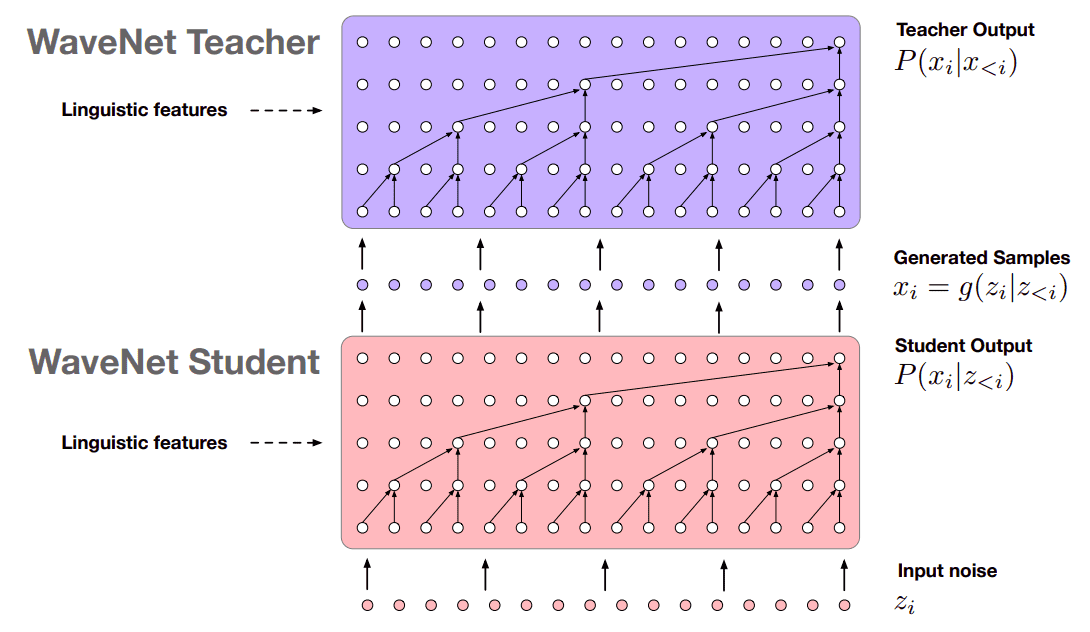 Overview of Probability Density Distillation. Source: Parallel WaveNet: Fast High-Fidelity Speech Synthesis
Parallel WaveNet is 1000 times faster than the original networks and can produce 20 seconds of audio in 1 second.
Also, note that similar techniques with IAFs to parallelize wave generation have also been used by other architectures such as ClariNet
Tacotron 2
Tacotron 2 improves and simplifies the original architecture. While there are no major differences, let’s see its key points:
The encoder now consists of 3 convolutional layers and a bidirectional LSTM replacing PreNets and CHBG modules
Location sensitive attention improved the original additive attention mechanism
The decoder is now an autoregressive RNN formed by a Pre-Net, 2 uni-directional LSTMs, and a 5-layer Convolutional Post-Net
A modified WaveNet is used as the Vocoder that follows PixelCNN++ and Parallel WaveNet
Mel spectrograms are generated and passed to the Vocoder as opposed to Linear-scale spectrograms
WaveNet replaced the Griffin-Lin algorithm used in Tacotron 1
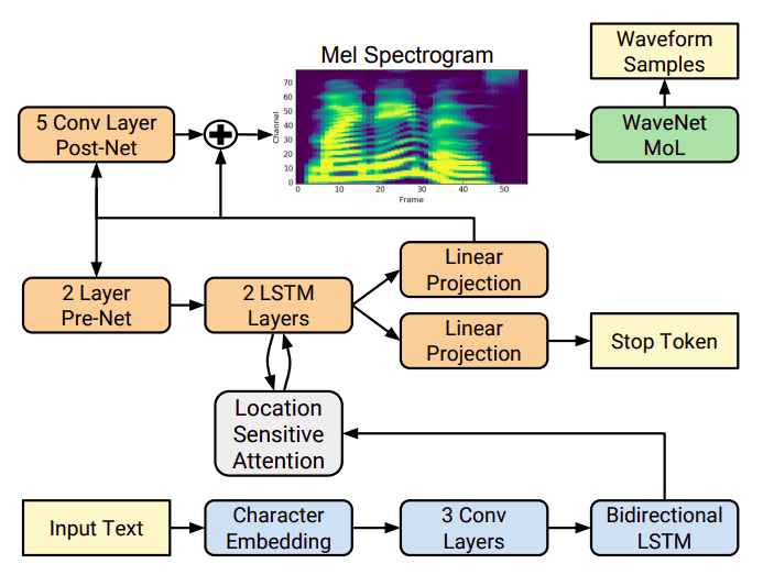 Tacotron 2. Source: Natural TTS Synthesis by Conditioning WaveNet on Mel Spectrogram Predictions
Tacotron 2 received an impressive MOS of 4.53.
Global Style Tokens (GST)
Global Style Tokens is a new idea to augment Tacotron-based architectures . The authors proposed a bank of embeddings that can be trained jointly with Tacotron in an unsupervised manner (also referred as GST-Tacotron). The embeddings represent the acoustic expressiveness of different speakers and are trained with no explicit labels. In other words, they aim to model different speaking styles.
 Source: Style Tokens: Unsupervised Style Modeling, Control and Transfer in End-to-End Speech Synthesis
During training, a reference encoder is used to extract a fixed-length vector which encodes the information about the speaking style (also known as prosody). This is then passed to the “style token layer”, an attention layer that calculates the contribution of each token to the resulting style embedding.
During inference, a reference audio sequence can be used to produce a style embedding or we can manually control the speech style.
TTS with Transformers
Transformers are dominating the Natural Language field for a while now, so it was inevitable that they will gradually enter the TTS field. Transformers-based models aim to tackle two problems of previous TTS methods such as Tacotron2:
Low efficiency during training and inference
Difficulty in modeling long dependencies using RNNs
The first transformers-based architecture introduced in 2018 and replaced RNNs with multi-head attention mechanisms that can be trained in parallel.
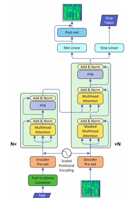 Source: Neural Speech Synthesis with Transformer Network
As you can see above, the proposed architecture resembles the Transformer proposed in the famous “Attention is all you need” paper. In more details we have:
A Text-to-Phoneme Converter: converts text to phonemes
Scaled positional encoding: they use a sinusoidal form that captures information about the position of phonemes
An Encoder Pre-Net: a 3-layer CNN similar to Tacotron 2, which learns the phonemes embeddings
A Decoder Pre-Net: consumes a mel spectogram and projects it into the same subspace as phoneme embeddings
The Encoder: The bi-directional RNN is replaced with a Transformer Encoder with multi-head attention
The Decoder: The 2-layer RNN with location-sensitive attention is replaced by a Transformer decoder with multi-head self-attention
Mel Liner and Stop Linear: Two different linear projections are used to predict the mel spectrogram and the stop token respectively
The Transformer-based system achieved a MOS of 4.39.
FastSpeech
A similar approach with Transformers is followed by FastSpeech. FastSpeech managed to speed up the aforementioned architecture by 38x. In short, this was accomplished by the following 3 things:
Parallel mel-specogram generation
Hard alignment between phonemes and their mel-spectograms in contrast to soft attention alignments in the previous model
A length regulator that can easily adjust voice speed by lengthening or shortening the phoneme duration to determine the length of the generated mel spectrograms,
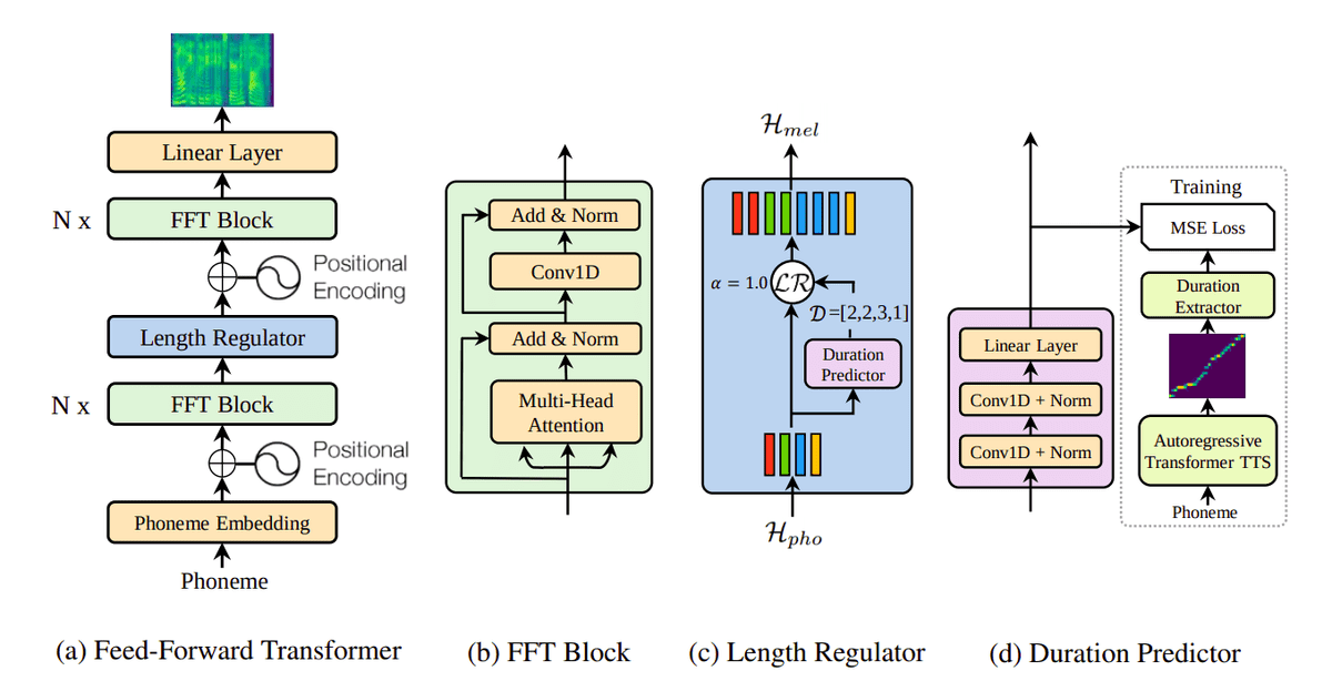 Source: FastSpeech: Fast, Robust and Controllable Text to Speech
In the same direction, Fast Speech 2 and FastPitch came later and improved upon the original idea.
Flow-based TTS
Before we examine flow-based TTS, let’s explain what flow-based models are. Contrary with GANs and VAEs which approximate the probability density function of our data , Flow-based models do exactly that with the help of normalizing flows.
Normalizing Flows are a method for constructing complex distributions by transforming a probability density through a series of invertible mappings. By repeatedly applying a predefined rule for change of variables, the initial density ‘flows’ through the sequence of invertible mappings. At the end of this sequence, we obtain a valid probability distribution and hence this type of flow is referred to as a normalizing flow. For more details, check out the original paper
A lot of models have been proposed based om that idea with the most popular being RealNVP, NICE and Glow. You can have a look at this excellent article by Lillian Weng to get a more complete understanding.
So as you may have guessed, Flow-based TTS models take advantage of this idea and apply it on speech synthesis.
WaveGlow
WaveGlow by Nvidia is one of the most popular flow-based TTS models. It essentially tries to combine insights from Glow and WaveNet in order to achieve fast and efficient audio synthesis without utilizing auto-regression. Note that WaveGlow is used strictly to generated speech from mel spectograms replacing WaveNets. They are not end-to-end TTS systems.
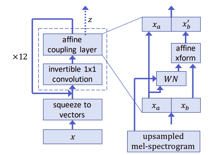 Waveglow. Source: WaveGlow: A Flow-based Generative Network for Speech Synthesis
The model is trained by minimizing the negative log-likelihood function of the data. To achieve that, we need to use Invertible Neural Networks because otherwise, the function is intractable. I won’t go into many details because we would need a separate article to explain everything but here are a few things to remember:
Invertible neural networks are usually constructed using coupling layers. In this case, the authors used affine coupling layers
They also used 1x1 invertible convolutions following the Glow paradigm
Once the model is trained, the inference is simply a matter of randomly sampling values and run them through the network
Similar models include Glow-TTS and Flow-TTS. Flowtron, on the other hand, uses an Autoregressive Flow-based Generative Network to generate speech. So we can see that there are research works in both areas of flow-based models.
GAN-based TTS and EATS
Finally, I’d like to close with one of the most recent and impactful works. End-to-End Adversarial Text-to-Speech by Deepmind.
EATS falls into the category of GAN-based TTS and is inspired by a previous work called GAN-TTS
EATS takes advantage of the adversarial training paradigm used in Generative Adversarial Networks. It operates on pure text or raw phoneme sequences and produces raw waveforms as outputs. EATS consists of two basic submodules: the aligner and the decoder.
The aligner receives the raw input sequence and produces low-frequency aligned features in an abstract feature space. The aligner’s job is to map the unaligned input sequence to a representation that is aligned with the output. The decoder takes the features and upsamples them using 1D convolutions to produce audio waveforms. The whole system is trained as a whole entity in an adversarial manner
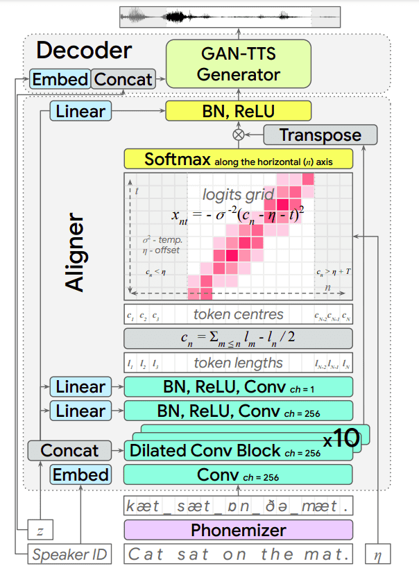 Source: End-to-End Adversarial Text-to-Speech
A few key things worth mentioning are:
The generator is a feed-forward neural network that uses a differentiable alignment scheme based on token length prediction
To allow the model to capture temporal variation in the generated audio, soft dynamic time warping is also employed.
As always for more details, please advise the original paper.
EATS achieved a MOS of 4.083
You can also find a great explanation of this architecture by Yannic Kilcher, on his Youtube channel.
Conclusion
Text to speech is an area of research with a lot of novel ideas. It is evident that the field has come a long way over the past few years. Take a look at smart devices such as Google assistant, Amazon’s Alexa and Microsoft’s Cortana.
If you want to experiment with some of the above models, all you have to do is go into Pytorch’s or TensorFlow model hub, find your model and play around with it. Another great resource is the following repo by Mozilla: TTS: Text-to-Speech for all. If you also want us to explore a different architecture, feel free to ping us and we can include it here as well.
References
- [1] Heiga Zen, Keiichi Tokuda, Alan W. Black, Statistical parametric speech synthesis, Speech Communication, Volume 51, Issue 11, 2009
- [2] Aaron van den Oord et al., WaveNet: A Generative Model for Raw Audio, arXiv:1609.03499, 2016
- [3] Sercan O. Arik et al., Deep Voice: Real-time Neural Text-to-Speech, arXiv:1702.07825, 2017
- [4] Paine et al. , Fast Wavenet Generation Algorithm, arXiv:1611.09482v1, 2016
- [5] Arik et al., Deep Voice 2: Multi-Speaker Neural Text-to-Speech, arXiv:1705.08947, 2017
- [6] Ping et al., Deep Voice 3: Scaling Text-to-Speech with Convolutional Sequence Learning, arXiv:1710.07654, 2017
- [7] Yuxuan Wang et al., Tacotron: Towards End-to-End Speech Synthesis, arXiv:1703.10135, 2017
- [8] Jonathan Shen et al., Natural TTS Synthesis by Conditioning WaveNet on Mel Spectrogram Predictions, arXiv:1712.05884, 2017
- [9] Aaron van den Oord et al., Parallel WaveNet: Fast High-Fidelity Speech Synthesis, arXiv:1711.10433, 2017
- [10] Yuxuan Wang et al., Style Tokens: Unsupervised Style Modeling, Control and Transfer in End-to-End Speech Synthesis, arXiv:1803.09017, 2018
- [11] Naihan Li et al., Neural Speech Synthesis with Transformer Network, arXiv:1809.08895, 2018
- [12] Yi Ren et al., FastSpeech: Fast, Robust and Controllable Text to Speech, arXiv:1905.09263, 2019
- [13] Yi Ren et al., FastSpeech 2: Fast and High-Quality End-to-End Text to Speech, arXiv:2006.04558, 2020
- [14] Ryan Prenger et al., WaveGlow: A Flow-based Generative Network for Speech Synthesis, arXiv:1811.00002, 2018
- [15] Jeff Donahue et al., End-to-End Adversarial Text-to-Speech, arXiv:2006.03575, 2020
* Disclosure: Please note that some of the links above might be affiliate links, and at no additional cost to you, we will earn a commission if you decide to make a purchase after clicking through.