Best Graph Neural Network architectures: GCN, GAT, MPNN and more

Traditionally, datasets in Deep Learning applications such as computer vision and NLP are typically represented in the euclidean space. Recently though there is an increasing number of non-euclidean data that are represented as graphs.

To this end, Graph Neural Networks (GNNs) are an effort to apply deep learning techniques in graphs. The term GNN is typically referred to a variety of different algorithms and not a single architecture. As we will see, a plethora of different architectures have been developed over the years. To give you an early preview, here is a diagram presenting the most important papers on the field. The diagram has been borrowed from a recent review paper on GNNs by Zhou J. et al¹.

Source: Graph Neural Networks: A Review of Methods and Applications¹

Before we dive into the different types of architectures, let’s start with a few basic principles and some notation.

Graph basic principles and notation

Graphs consist of a set of nodes and a set of edges. Both nodes and edges can have a set of features. From now on, a node’s feature vector will be denoted as $h_i$ , where $i$ is the node’s index. Similarly an edge’s feature vector will be denoted as $e_{ij}$ , where $i$ , $j$ are the nodes that the edge is attached to.

As you might also know, graphs can be directed, undirected, weighted and weighted. Thus each architecture may be applied only to a type of graph or to all of them.

So can we start developing a Graph Neural Network?

The basic idea behind most GNN architectures is graph convolution. In essence, we try to generalize the idea of convolution into graphs. Graphs can be seen as a generalization of images where every node corresponds to a pixel connected to 8 (or 4) adjacent neighbours. Since CNNs take advantage of convolution with such great success, why not adjust this idea into graphs?

Graph convolution

Graph convolution predicts the features of the node in the next layer as a function of the neighbours’ features. It transforms the node’s features $x_i$ in a latent space $h_i$ that can be used for a variety of reasons.

x_i -> h_i

Visually this can be represented as follows:

But what can we actually do with these latent node features vectors? Typically all applications fall into one of the following categories:

Node classification
Edge classification
Graph classification

Node classification

If we apply a shared function $f$ to each of the latent vectors $h_i$ , we can make predictions for each of the nodes. That way we can classify nodes based on their features:

Z_i=f(h_i)

Edge classification

Similarly, we can use it to classify edges based on their features. To accomplish this, we generally need both the adjacent node vectors as well as the edge features if they exist. Mathematically we have:

Z_{ij}=f(h_i, h_j, e_{ij})

Graph classification

Lastly, we can predict some attribute for the entire graph by aggregating all node features and applying an appropriate function $f$ .

Z_G=f(\sum_i{h_i})

The aggregation usually is a permutation-invariant function such as a sum, mean operation, a pooling operation or even a trainable linear layer.

Inductive vs Transductive learning

A terminology that can be confusing is the notion of inductive vs transductive, which is used often in the GNNs literature. So let’s clarify it before we proceed.

In transductive learning, the model has already encountered both the training and the test input data. In our case these are the nodes of a large graph where we want to predict the node labels. If a new node is added to the graph, we need to retrain the model.

In inductive learning, the model sees only the training data. Thus the generated model will be used to predict graph labels for unseen data.

To understand that from the GNNs perspective, imagine the following example. Suppose that we have a graph with 10 nodes. Also consider that the structure of the graph, how nodes are connected, is not important for the following example. We use 6 of them for the training set (with the labels) and 4 for the test set. How do we train this model?

Use a semi-supervised learning approach and train the whole graph using only the 6 labeled data points. This is called inductive learning. Models trained correctly with inductive learning can generalize well but it can be quite hard to capture the complete structure of the data.
Use a self-supervised approach which will label the unlabeled data points using additional information and train the model on all 10 nodes. This is called transductive learning and is quite common in GNNs since we use the whole graph to train the model.

With that out of the way, let’s now proceed with the most popular GNN architectures.

Spectral methods

Spectral methods deal with the representation of a graph in the spectral domain. The idea is quite intuitive.

These methods are based on graph signal processing and define the convolution operator in the spectral domain using the Fourier transform $F$ . The graph signal $x$ is initially transformed to the spectral domain by the graph Fourier transform $F$ . Then the convolution operation is conducted by doing an element-wise multiplication. After the convolution, the resulting signal is transformed back using the inverse graph Fourier transform $F^{-1}$ .

F(x) = U^T x

F^{-1}(x) = U x

$U$ is a matrix defined by the eigenvectors of $L$ , where $L= U\Lambda U^T$ . $\Lambda$ is a diagonal matrix with the eigenvalues of the graph $\Lambda = diag([\lambda0, . . . , \lambda1])$

The convolution operation is defined as:

g*x = F^{-1}(F(g) \cdot F(x)) = U ( U^Tg \cdot U^Tx)

$L$ is the normalized graph Laplacian and is constructed as depicted below:

L = I -D^{-\frac{1}{2}}AD^{-\frac{1}{2}}

$U^Tg$ is the filter in the spectral domain, $D$ is the degree matrix and $A$ is the adjacency matrix of the graph. For a more detailed explanation, check out our article on graph convolutions.

Spectral Networks

Spectral networks² reduced the filter in the spectral domain to be a diagonal matrix $g_w$ where $w$ are the learnable parameters of the network. As a result, one can build a network that learns convolutional filters for graph classification. Drawbacks?

The filter is applied on the entire graph so there is not a notion of locality that we have in images.
It is computationally inefficient, especially for big graphs.

ChebNets

To solve the problem of locality, ChebNets³ propose that the feature representation of any vector should be affected only by his k-hop neighborhood. Using Chebyshev expansion of order K, we can define a K-localized convolution that can be used to form a convolutional neural network.

This results in lower computational complexity since we don’t need to compute the eigenvectors of the Laplacian. The convolution is now computed using Chebyshev polynomials.

Graph Convolutional Networks (GCN)

Graph Convolutional Networks (GCN)⁴ is the most cited paper in the GNN literature and the most commonly used architecture in real-life applications. In GCNs, the K-localized convolution proposed in ChebNets is simplified to $K=1$ .

They proposed the following changes:

1) They enforce self-connections by adding the identity matrix $I$ to the adjacency matrix $A$ .

\tilde{A} = A + I

2) They used the symmetric normalization of the Laplacian $L$ .

L_{norm} = D^{-\frac{1}{2}}LD^{-\frac{1}{2}} = I - D^{-\frac{1}{2}}AD^{-\frac{1}{2}}

3) They used a renormalization trick to solve exploding/vanishing gradient problems.

I + D^{-\frac{1}{2}}AD^{-\frac{1}{2}} \rightarrow \tilde{D}^{-\frac{1}{2}}\tilde{A}\tilde{D}^{-\frac{1}{2}}

where $\tilde{D}_{ij}$ is the degree matrix of the graph. $\tilde{D}_{ij}$ performs a row-wise summation of the adjacency matrix $\tilde{D}_{ij} = \sum_j \tilde{A}_{ij}$ , which produces the degree of each node.

Based on the above, if $H$ is the feature matrix and $W$ the trainable weight matrix, the update rule for the GCN layer becomes the following:

H^{(l+1)} = \sigma (\tilde{D}^{-\frac{1}{2}}\tilde{A}\tilde{D}^{-\frac{1}{2}} H^{(l)}W^{(l)})

From a node-wise perspective, the update rule can be written as :

h^{(l)}_i = \sigma( \sum_{i \in N_j} c_{ij} W h_j)

Where $c_{ij}= \frac{1}{\sqrt{|N_i| |N_j|}}$ , and $N_i$ and $N_j$ are the sizes of the nodes’ neighbourhoods.

GCNs are much more computationally effective than their predecessors and simpler to code (see our colab notebook), but they have a few limitations.

They don’t directly support edge features.
They omit the notion of messages in graphs. Typically, nodes can send messages (numeric vectors) along graph edges.

Graph Convolutional Network. Source: Semi-Supervised Classification with Graph Convolutional Networks⁴

Spatial methods

Spatial approaches define convolutions directly on the graph based on the graph topology. They usually follow the same pattern:

The node’s feature vectors are transformed using some sort of projection.
They are aggregated by a permutation-invariant function.
The feature vector of each node is updated based on its current values and the aggregated neighbourhood representation.

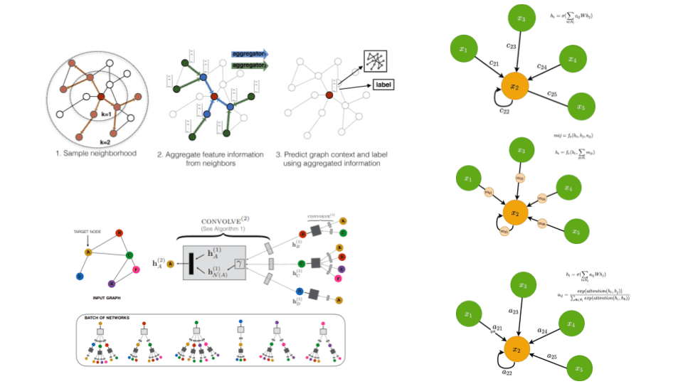
Message Passing Neural Networks (MPNN)

Message Passing Neural Networks⁵ utilize the notion of messages in GNNs. A message $m_{ij}$ can be sent across edges $i$ and $j$ and is computed using a message function $f_e$ . $f_e$ is generally a small MLP and is taking into consideration both the nodes’ and edge’s features. Mathematically, for two nodes $i$ and $j$ with edge features $e_{ij}$ we have the following:

m_{ij} = f_e(h_i,h_j,e_{ij})

All messages arriving at each node are then aggregated using a permutation-invariant function, such as summation. The aggregated representation is then combined with the existing node features via $f_v$ (another MLP), resulting in an updated node feature vector. Mathematically, this will look like this:

h_i = f_v (h_{i}, \sum_{j \in N_i} m_{ji})

MPNNs are a powerful framework and are considered one of the most generic GNN architectures. However, they do occasionally suffer from scalability issues. Why? Because they require to store and process edge messages as well as the node features. That’s why in practice, it’s applicable only for small-ish graphs.

Graph Attention Networks (GAT)

To understand Graph Attention Networks⁶, let’s revisit the node-wise update rule of GCNs. As you can see, we have this coefficient $\frac{1}{\sqrt{|N_i| |N_j|}}$ which is multiplied in our projection of the node features. The coefficient is derived from the degree matrix of the graph and is heavily dependent on the structure of the graph. Intuitively, it represents how important the node’s $j$ features are for node $i$ .

h^{(l)}_i = \sigma( \sum_{i \in N_j} \frac{1}{\sqrt{|N_i| |N_j|}} W h_j)

The main idea behind GAT is to compute that coefficient implicitly rather than explicitly as GCNs do. That way we can use more information besides the graph structure to determine each node’s “importance”. How? By considering the coefficient to be a learnable attention mechanism.

The authors behind GAT proposed that the coefficient, from now on denoted as $a_{ij}$ , should be computed based on node features, which are then passed into an attention function. Note that edge features can also be included. Finally, the softmax function is applied in the attention weights $a_{ij}$ to that result in a probability distribution. Mathematically we have:

a_{ij}= attention(h_i,h_j)

a_{ij}= \frac{exp(a_{ij})}{\sum_{k \in N_i}exp(a_{ik})}

Visually this can be seen on the left side of the following image

Attention in GAT. Left: The attention mechanism. Right: An illustration of multihead attention on its neighborhood. Source: Graph Attention Networks⁶

The update rule is now formed as follows:

h^{(l)}_i = \sigma( \sum_{i \in N_j} a_{ij} W h_j)

A few important notes before we continue:

GATs are agnostic to the choice of the attention function. In the paper, the authors used the additive score function as proposed by Bahdanau et al.
Multi-head attention is also incorporated with success. As shown in the right side of the image above, they compute simultaneously $K=3$ different attention heads and then concatenate the features to obtain the new feature vector.
The coefficient does not depend on the graph structure. Only on the node representations.
GATs are fairly computationally efficient.
The work can be extended to include edge features as well.
They are quite scalable.

Sampling methods

One major drawback of most GNN architectures is scalability. In general, each node’s feature vector depends on its entire neighbourhood. This can be quite inefficient for huge graphs with big neighbourhoods. To solve this issue, sampling modules have been incorporated. The main idea of sampling modules is that instead of using all neighbourhood information, we can sample a subset of them to conduct propagation.

GraphSage

GraphSage⁷ popularized this idea by proposing the following framework:

Sample uniformly a set of nodes from the neighbourhood .
Aggregate the feature information from sampled neighbours.
Based on the aggregation, we perform graph classification or node classification.

GraphSage process. Source: Inductive Representation Learning on Large Graphs ⁷

On each layer, we extend the neighbourhood depth $K$ , resulting in sampling node features K-hops away. This is similar to increasing the receptive field of classical convnets. One can easily understand how computationally efficient this is compared to using the entire neighbourhood. That concludes the forward propagation of GraphSage.

The key contribution, though, of the GraphSage paper is how they actually trained the model. The authors actually proposed two basic ideas:

Train the model in a fully unsupervised way. This can be done by using a loss function which enforces nearby nodes to have similar representations and disparate nodes to have distinct representations.
We can also train in a supervised manner using labels and a form of cross entropy to learn the node representations

The tricky part is that we also train the aggregation function alongside with our learnable weight matrices. The authors experimented with 3 different aggregation functions: a) a mean aggregator, b) an LSTM aggregator and c) amax-pooling aggregator. In all 3 cases, the functions contain trainable parameters that are learned during training. This way the network will teach itself the “correct” way to aggregate the features from the sampled nodes.

PinSAGE

PinSAGE⁸ is a direct continuation of GraphSAGE and one of the most popular GNNs applications. PinSAGE is basically GraphSAGE applied in a very large graph (3 billion nodes and 18 billion edges). It is proposed by Pinterest and it is used in their recommendation system.

Besides their tremendous engineering effort, which is a big part of the paper and we’ll not cover here, let’s briefly see the main principles of the architecture:

They define the node’s neighbourhood using random walks. By simulating random walks starting from target nodes, they can choose the top nodes with the highest visit counts. One side effect is that now each node is assigned with an importance score that indicates how important it is for the target node.
The aggregation is performed using “importance sampling”. In importance sampling, we simply normalize and sum up the importance scores generated by the random walks.
The model is trained in a supervised fashion on a dataset of nodes connected based on the users historic engagement on Pinterest.

PinSAGE overview. Source: Graph Convolutional Neural Networks for Web-Scale Recommender Systems⁸

Dynamic Graphs

Dynamic graphs are graphs whose structure keeps changing over time. That includes both nodes and edges, which can be added, modified and deleted. Examples include social networks, financial transactions and more. A dynamic graph can be represented as an ordered list or a stream of time-stamped events that change the graph’s structure.

ML research on dynamic graphs is very new but there are a few notable architectures.

Temporal Graph Networks (TGN)

The most promising architecture is Temporal Graph Networks⁹. Since dynamic graphs are represented as a timed list, the node’s neighbourhoods are changing over time. At each time $t$ , we can get a snapshot of the graph. The neighbourhood at a particular time $t$ is called a temporal neighbourhood.

As you can see in the following image, the goal of TGN is to predict the node embeddings at a particular timestamp. These embeddings can be fed into a Decoder network that will perform the task at hand.

Example of a TGN encoder ingesting a dynamic graph. Source: Deep learning on dynamic graphs by Emanuele Rossi and Michael Bronstein

The architecture is proposed by Twitter and is trained on their tweets graph. The nodes represent the tweets and the edges the interactions between them. The goal of the model is to predict the interactions that haven’t yet happened at timestamp $t$ in the form of probability. In other words, they performed an edge prediction. The network is trained in a self-supervised fashion: during each epoch, the encoder processes the events in chronological order and predicts the next interaction based on the previous ones.

But how exactly does the TGN encoder look like?

The main component is a GAT network that produces the node embeddings. The GAT module receives information in two forms:

The node features of the temporal neighbourhood at a particular time. We simply pass the features from the neighbourhood to the GAT module, which will transform them, aggregate them, and update the hidden representations.
The node’s memory. The node’s memory is a compact representation of the node’s past interactions. Each node has a different representation for each timestamp. The memory is updated using messages, as we described in MPNNs. All the messages from different nodes are aggregated and processed by the memory module which is usually implemented as a Recurrent Neural Network (RNN).

Temporal Graph Network. Source: Temporal Graph Networks for Deep Learning on Dynamic Graphs⁹

Conclusion

GNNs are a very active, new field of research that has a tremendous potential, because there are many datasets in real-life applications that can be structured as graphs. In the following articles, we will utilize Pytorch Geometric to play around with graphs and build our own GNN.

Until then, let me recommend a few resources if you want to dive deeper. A very good introductory video is a lecture by Petar Veličković on the Theoretical Foundations of Graph Neural Networks. For a more comprehensive understanding of the aforementioned papers, check out the excellent video series by Aleksa Gordić on his AI Epiphany channel.

If you find our work useful and want us to continue writing, consider supporting us by making a small donation or buying our course. See you next time.

Cite as

@article{karagiannakos2021gnnarchitectures,
    title   = "Best Graph Neural Networks architectures:  GCN, GAT, MPNN and more",
    author  = "Karagiannakos, Sergios",
    journal = "https://theaisummer.com/",
    year    = "2021",
    howpublished = {https://theaisummer.com/gnn-architectures/},
  }

References

* Disclosure: Please note that some of the links above might be affiliate links, and at no additional cost to you, we will earn a commission if you decide to make a purchase after clicking through.

References

- Zhou, Jie, et al. “Graph Neural Networks: A Review of Methods and Applications.” AI Open, vol. 1, Jan. 2020, pp. 57–81. ScienceDirect↩
- Bruna, Joan, et al. “Spectral Networks and Locally Connected Networks on Graphs.” ArXiv:1312.6203 [Cs], May 2014↩
- Defferrard, Michaël, et al. “Convolutional Neural Networks on Graphs with Fast Localized Spectral Filtering.” ArXiv:1606.09375 [Cs, Stat], Feb. 2017↩
- Kipf, Thomas N., and Max Welling. “Semi-Supervised Classification with Graph Convolutional Networks.” ArXiv:1609.02907 [Cs, Stat], Feb. 2017↩
- Gilmer, Justin, et al. “Neural Message Passing for Quantum Chemistry.” ArXiv:1704.01212 [Cs], June 2017↩
- Veličković, Petar, et al. “Graph Attention Networks.” ArXiv:1710.10903 [Cs, Stat], Feb. 2018↩
- Hamilton, William L., et al. “Inductive Representation Learning on Large Graphs.” ArXiv:1706.02216 [Cs, Stat], Sept. 2018↩
- Ying, Rex, et al. “Graph Convolutional Neural Networks for Web-Scale Recommender Systems.” ArXiv:1806.01973 [Cs, Stat], June 2018↩
- Rossi, Emanuele, et al. “Temporal Graph Networks for Deep Learning on Dynamic Graphs.” ArXiv:2006.10637 [Cs, Stat], Oct. 2020↩