JAX for Machine Learning: how it works and why learn it

JAX is the new kid in Machine Learning (ML) town and it promises to make ML programming more intuitive, structured, and clean. It can possibly replace the likes of Tensorflow and PyTorch despite the fact that it is very different in its core.

As a friend of mine said, we had all sorts of Aces, Kings, and Queens. Now we have JAX.

In this article, we will explore what is JAX and why one should use it over all the other libraries. We will make our points using code snippets that capture the power of JAX and we will present some good-to-know features of it.

If that sounds interesting, hop in.

What is Jax?

Jax is a Python library designed for high-performance ML research. Jax is nothing more than a numerical computing library, just like Numpy, but with some key improvements. It was developed by Google and used internally both by Google and Deepmind teams.

Source: JAX documentation

Install JAX

Before we discuss the main advantages of JAX, I suggest you to install JAX in your Python environment or in a Google colab so you can follow along and run the code by yourself. Of course, I will leave a link to the full code at the end of the article.

To install JAX, we can simply use pip from our command line:

$ pip install --upgrade jax jaxlib

Note that this will support execution-only on CPU. If you also want to support GPU, you first need CUDA and cuDNN and then run the following command (make sure to map the jaxlib version with your CUDA version):

$ pip install --upgrade jax jaxlib==0.1.61+cuda110 -f https://storage.googleapis.com/jax-releases/jax_releases.html

For troubleshooting, check the official Github instructions.

Now let’s import JAX alongside Numpy. We will use Numpy to compare different use cases.

import jax
import jax.numpy as jnp
import numpy as np

JAX basics

Let’s start with the basics. As we already told, JAX’s main and only purpose is to perform numeric operations in an expressible and high-performance way. This means that the syntax is almost identical to Numpy. For example, if we want to create an array of zeros, we’d have:

x = np.zeros(10)

y= jnp.zeros(10)

The difference lies behind the scenes.

The DeviceArray

You see one of JAX’s main advantages is that we can run the same program, without any change, in hardware accelerators like GPUs and TPUs.

This is accomplished by an underlying structure called DeviceArray, which essentially replaces Numpy’s standard array.

DeviceArrays are lazy, which means that they keep the values in the accelerator and pull them only when needed.

x
# array([0., 0., 0., 0., 0., 0., 0., 0., 0., 0.])

y
# DeviceArray([0., 0., 0., 0., 0., 0., 0., 0., 0., 0.], dtype=float32)

We can use DeviceArrays just like we use standard arrays. We can pass it to other libraries, plot graphs, perform differentiation and things will work. Also note that the majority of Numpy’s API (functions and operations) are supported by JAX, so your JAX code will be almost identical to Numpy.

The other big thing is speed. Well JAX is faster. Much faster. Let’s look at a simple example. We create two arrays with size (1000, 1000), one with Numpy and one with JAX, and we calculate the inner product with itself.

Let’s timeit the two operations

x = np.random.rand(1000,1000)
y = jnp.array(x)

%timeit -n 1 -r 1 np.dot(x,x)
# 1 loop, best of 1: 52.6 ms per loop

%timeit -n 1 -r 1 jnp.dot(y,y).block_until_ready()
# 1 loop, best of 1: 1.47 ms per loop

Impressive right? Well, it’s expected. The calculations are faster in the GPUs. Also did you notice the block_until_ready() function. Because JAX is asynchronous, we need to wait until the execution is complete in order to properly measure the time.

You can’t possibly believe that this is all JAX has to offer, right?

Now for the good stuff...

Why JAX?

If speed and automatic support for GPUs aren't enough for you, I don’t blame you. It seems that every other library can handle those. To further understand the benefits of JAX, we have to dive deeper. JAX can be seen as a set of function transformations of regular Python and Numpy code.

An example of such transformations is differentiation. Does JAX support automatic differentiation?

I’m sure you guessed it correctly.

Auto differentiation with grad() function

JAX is able to differentiate through all sorts of python and NumPy functions, including loops, branches, recursions, and more.

This is incredibly useful for Deep Learning apps as we can run backpropagation pretty much effortlessly. The main function to accomplish this is called grad(). Here is an example. We define a simple quadratic function and take its derivative on point 1.0.

In order to prove that the result it’s correct, we will compute the derivative manually as well.

from jax import grad

def f(x):
  return 3*x**2 + 2*x + 5

def f_prime(x):
  return 6*x +2

grad(f)(1.0)
# DeviceArray(8., dtype=float32)

f_prime(1.0)
# 8.0

A very surprising thing to me was that JAX is actually doing analytical gradient solve under the hood instead of some other fancy technique. It simply takes the form of the function and performs the chain rule. Since automatic differentiation is so much more than that, I highly recommend looking at the official documentation for a more complete understanding.

Accelerated Linear Algebra (XLA compiler)

One of the factors that make JAX so fast is also Accelerated Linear Algebra or XLA.

XLA is a domain-specific compiler for linear algebra that has been used extensively by Tensorflow.

In order to perform matrix operations as fast as possible, the code is compiled into a set of computation kernels that can be extensively optimized based on the nature of the code.

Example of such optimizations include:

Fusion of operations: Intermediate results are not saved into memory
Optimized layout: Optimize the “shape” an array is represented in memory

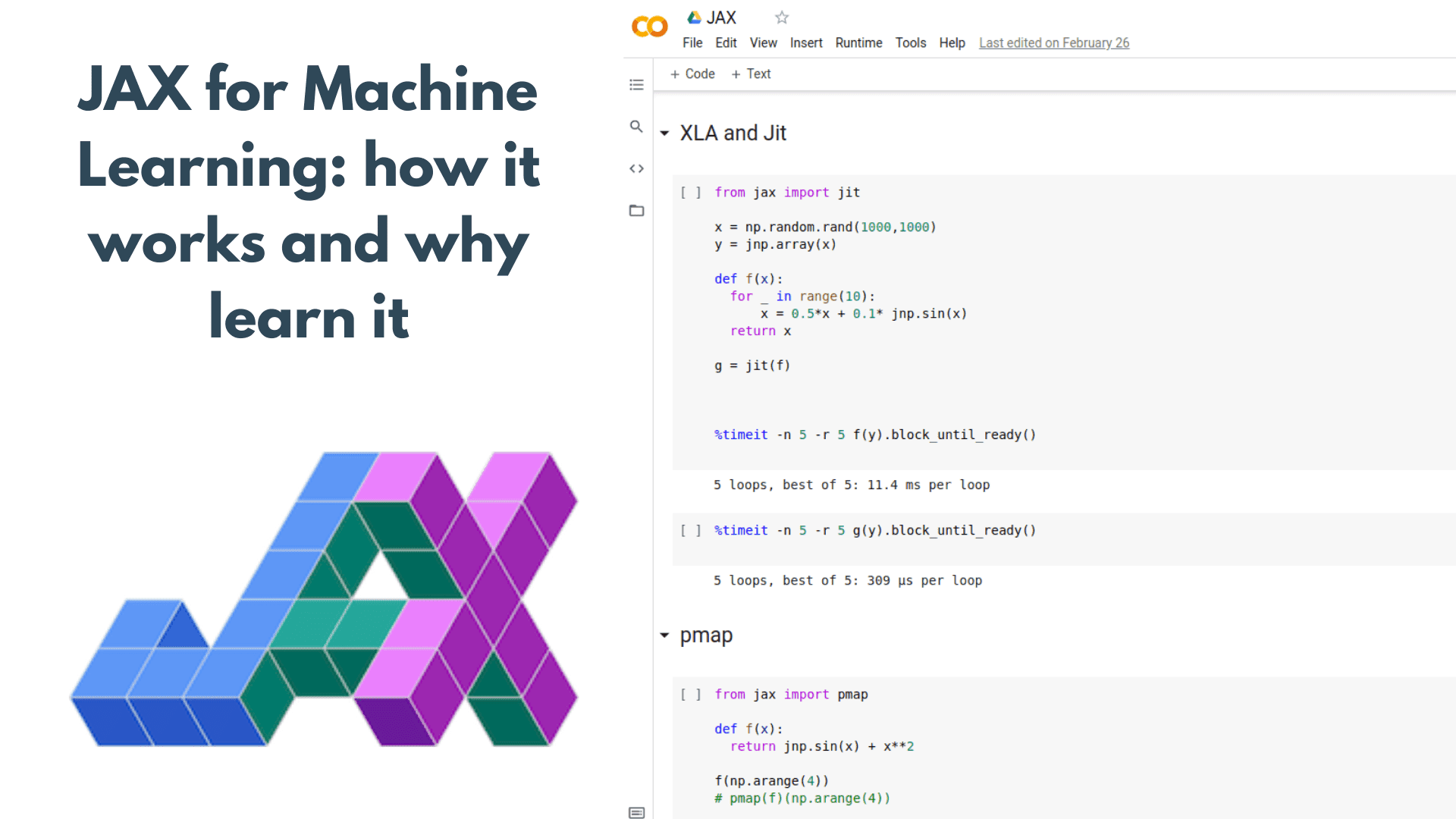
Just in time compilation (jit)

Just in time compilation comes hand in hand with XLA. In order to take advantage of the power of XLA, the code must be compiled into the XLA kernels. This is where jit comes into play.

Just-in-time (JIT) compilation is a way of executing computer code that involves compilation during the execution of a program – at run time – rather than before execution.

In order to use XLA and jit, one can use either the jit() function or the @jit annotation.

from jax import jit

x = np.random.rand(1000,1000)
y = jnp.array(x)

def f(x):

  for _ in range(10):
      x = 0.5*x + 0.1* jnp.sin(x)

  return x

g = jit(f)

%timeit -n 5 -r 5 f(y).block_until_ready()
# 5 loops, best of 5: 10.8 ms per loop

%timeit -n 5 -r 5 g(y).block_until_ready()
# 5 loops, best of 5: 341 µs per loop

Once again the improvement in execution time is more than obvious. Of course, jit can also be combined with grad transformation (or any other transformation for that matter), making backpropagation super fast.

Also, note that jit has some shortcomings: for example, if it can’t accurately represent the function (which usually happens with “if” branches), it will likely fail. However, for the most use cases related to deep learning, it is incredibly useful.

Replicate computation across devices with pmap

Pmap is another transformation that enables us to replicate the computation into multiple cores or devices and execute them in parallel(p in pmap stands for parallel) .

It automatically distributes computation across all the current devices and handles all the communication between them. To inspect the available devices, you can run jax.devices().

from jax import pmap

def f(x):
  return jnp.sin(x) + x**2

f(np.arange(4))
#DeviceArray([0.       , 1.841471 , 4.9092975, 9.14112  ], dtype=float32)

pmap(f)(np.arange(4))
#ShardedDeviceArray([0.       , 1.841471 , 4.9092975, 9.14112  ], dtype=float32)

Note that the DeviceArray has now become ShardedDeviceArray, which is the structure that handles the parallel execution.

Another very cool thing that JAX allows us to do is collective communication between devices. Let’s say that we want to perform a “reduce” operation between the values on all devices (for example take the sum). To perform that, we need to gather all the data from all devices and execute the sum. This can easily be accomplished as follows:

from functools import partial
from jax.lax import psum

@partial(pmap, axis_name="i")
def normalize(x):

  return x/ psum(x,'i')

normalize(np.arange(8.))

The above code maps the vector x across all devices and runs a collective communication operation to execute the psum (parallel sum). In other words, it collects all “x” from the devices, sums them up, and returns the result to each device to continue with the parallel computation. I borrowed the above example from this awesome talk by Matthew Johnson during GTC 2020.

You can also imagine that with pmap we can define our own computation patterns and exploit our devices in the best possible way. Just like we usually do with CUDA for individual cores, but this time is for separate devices.

Automatic vectorization with vmap

Vmap is, as the name suggests, a function transformation that enables us to vectorize functions (v stands for vector!).

We can take a function that operates on a single data point and vectorize it so it can accept a batch of these data points (or a vector) of arbitrary size. Here is an example:

from jax import vmap

def f(x):

  return jnp.square(x)

f(jnp.arange(10))

#DeviceArray([ 0,  1,  4,  9, 16, 25, 36, 49, 64, 81], dtype=int32)

vmap(f)(jnp.arange(10))

#DeviceArray([ 0,  1,  4,  9, 16, 25, 36, 49, 64, 81], dtype=int32)

You may wonder what we have gained here. To understand that, let’s take a peek at what happens when f(x) executes without the vmap:

An output list is initialized.
The square of 0 is computed and returned.
The result 0 is appended to the list.
The square of 1 is computed and returned.
The result 1 is appended to the list.
The square of 2 is computed and returned.
The result 4 is appended to the list.
And so on…

What vmap does is that it performs the square operation only once, because it batches all the values together and passes them through the function. And of course, this results in an increase both in speed and memory consumption.

While the aforementioned transformations are the ones that you definitely need to know, I would like to mention a few more things that surprised me during my JAX journey.

Pseudo-Random number generator

JAX’s random number generator works slightly differently than Numpy’s. Instead of being a standard stateful PseudoRandom Number Generator (PRNGs) as in Numpy and Scipy, JAX random functions all require an explicit PRNG state to be passed as a first argument.

A random number generator has a state. The next "random" number is a function of the previous number and the seed/state. The sequence of random values is finite and does repeat.

An important thing to notice is that PRNGs are working well both in terms of vectorization and parallel computation between devices

from jax import random

key = random.PRNGKey(5)

random.uniform(key)

Asynchronous dispatch

Another aspect of JAX that impressed me is that it uses asynchronous dispatch. This means that it does not wait for the operations to complete before returning control to the Python program. Instead, it returns a DeviceArray which is a future (just like Completable future in Java)

A future is a value that will be produced in the future on an accelerator device but isn’t necessarily available immediately.

The future can be passed to other operations without waiting for the computation to be completed. That way JAX allows Python code to run ahead of the accelerator, ensuring that it can enqueue operations for the hardware accelerator (e.g. GPU) without it having to wait.

Profiling JAX and Device memory profiler

The last feature I want to mention is profiling. You will be pleased to know that Tensoboard supports JAX profiling.

![Tensorboard JAX profiling](Tensorboard JAX profiling.png) Source: JAX Documentation

The same is true for Nvidia’s Nsight, which is used to debug and profile GPU code. Alongside, one can also use JAX’s built-in Device Memory Profiler, which provides visibility into how the JAX code executes on GPUs and TPUs. Here is a snippet from the documentation:

import jax
import jax.numpy as jnp
import jax.profiler

def func1(x):
  return jnp.tile(x, 10) * 0.5

def func2(x):
  y = func1(x)
  return y, jnp.tile(x, 10) + 1

x = jax.random.normal(jax.random.PRNGKey(42), (1000, 1000))

y, z = func2(x)

z.block_until_ready()

jax.profiler.save_device_memory_profile("memory.prof")

If you have installed pprof, a library by Google, you can execute the following command, which will open a browser window with all the necessary information.

$ pprof --web memory.prof

![Device Memory Profiling](Device Memory Profiling.png) Source: JAX documentation

Is this awesome or what?

Feel free to play around with it. I know I did.

Conclusion

In this post, I tried to give an overview of JAX’s benefits over other libraries and present simple code snippets to learn its basic syntax and intricacies. By the way, you can find the full code in this colab notebook or in our github repository.

In the next articles, we will take it a step further and explore how to build and train deep neural nets with JAX, as well as have a peek at the different frameworks built on top of it.

If you find this article interesting, don’t forget to share it on social media.

References

* Disclosure: Please note that some of the links above might be affiliate links, and at no additional cost to you, we will earn a commission if you decide to make a purchase after clicking through.

References

JAX: Accelerated Machine Learning Research , SciPy 2020 , VanderPlas
JAX: accelerated machine learning research via composable function transformations in Python