Intuitive Explanation of Skip Connections in Deep Learning

Nowadays, there is an infinite number of applications that someone can do with Deep Learning. However, in order to understand the plethora of design choices such as skip connections that you see in so many works, it is critical to understand a little bit of the mechanisms of backpropagation.

If you were trying to train a neural network back in 2014, you would definitely observe the so-called vanishing gradient problem. In simple terms: you are behind the screen checking the training process of your network and all you see is that the training loss stop decreasing but it is still far away from the desired value. You check all your code lines to see if something was wrong all night and you find no clue. Not the best experience in the world, believe me!

The update rule and the vanishing gradient problem

So, let’s remind our self's the update rule of gradient descent without momentum, given L to be the loss function and $\lambda$ the learning rate:

w_{i}' = w_{i} + \Delta w_{i}

where $\Delta w_{i} = - \lambda \frac{\partial L}{\partial \Delta w_{i}}$

What is basically happening is that you try to update the parameters by changing them with a small amount $\Delta w_{i}$ that was calculated based on the gradient, for instance, let’s suppose that for an early layer the average gradient 1e-15 (ΔL/δw). Given a learning rate of 1e-4 ( λ in the equation), you basically change the layer parameters by the product of the referenced quantities, which is 1e-19 ( $\Delta w_{i}$ ). As a results, you don’t actually observe any change in the model while training your network. This is how you can observe the vanishing gradient problem.

Looking a little bit in the theory, one can easily grasp the vanishing gradient problem from the backpropagation algorithm. We will briefly inspect the backpropagation algorithm from the prism of the chain rule, starting from basic calculus to gain an insight on skip connections.

In short, backpropagation is the “optimization-magic” behind deep learning architectures. Given that a deep network consists of a finite number of parameters that we want to learn, our goal is to iteratively optimize these parameters with respect to the loss function L.

As you have seen, each architecture has some input (i.e. an image) and produces an output (prediction). The loss function is heavily based on the task we want to solve. For now, what you need to know is the loss function is a quantitative measure of the distance between two tensors, that can represent an image label, a bounding box in an image, a translated text in another language etc. You usually need some kind of supervision to compare the network’s prediction with the desired outcome (ground truth). Keep in mind that backpropagation belongs in the supervised machine learning category.

So, the beautiful idea of backpropagation is to gradually minimize this loss by updating the parameters of the network. But how can you propagate the scalar measured loss inside the network? That’s exactly where backpropagation comes into play.

Backpropagation and partial derivatives

In simple terms, backpropagation is about understanding how changing the weights (parameters) in a network changes the loss function by computing the partial derivatives. For the latter, we use the simple idea of the chain rule, to minimize the distance in the desired predictions. In other words, backpropagation is all about calculating the gradient of the loss function while considering the different weights within that neural network, which is nothing more than calculating the partial derivatives of the loss function with respect to model parameters. By repeating this step many times, we will continually minimize the loss function until it stops reducing, or some other predefined termination criteria are met.

Chain rule

The chain rule basically describes the gradient (change) of a loss function i.e. z with respect to some neural network parameter, let’s say x and y which are functions of a previous layer parameter t. Let f, g, h be different layers on the network that perform a non-linear operation in the input vector.

z = f(x,y) \quad x = g(t) \quad y = h(t)

Now, suppose that you are learning calculus and you want to express the gradient of z with respect to the input. This is what you learn in multi-variable calculus:

\frac{\partial z}{\partial t } = \frac{\partial f}{\partial x} \frac{\partial x}{\partial t} + \frac{\partial f}{\partial y} \frac{\partial y}{\partial t}

Interestingly, the famous algorithm does exactly the same operation but in the opposite way: it starts from the output z and calculates the partial derivatives of each parameter, expressing it only based on the gradients of the later layers.

It’s really worth noticing that all these values are often less than 1, independent of the sign. In order to propagate the gradient to the earlier layer’s, backpropagation uses multiplication of the partial derivatives (as in the chain rule). In general, multiplication with absolute value less than 1 is nice because it provides some sense of training stability, although there is not a strict mathematic theorem about that. However, one can observe that for every layer that we go backwards in the network the gradient of the network gets smaller and smaller.

Skip connections for the win

At present, skip connection is a standard module in many convolutional architectures. By using a skip connection, we provide an alternative path for the gradient (with backpropagation). It is experimentally validated that this additional paths are often beneficial for the model convergence. Skip connections in deep architectures, as the name suggests, skip some layer in the neural network and feeds the output of one layer as the input to the next layers (instead of only the next one).

As previously explained, using the chain rule, we must keep multiplying terms with the error gradient as we go backwards. However, in the long chain of multiplication, if we multiply many things together that are less than one, then the resulting gradient will be very small. Thus, the gradient becomes very small as we approach the earlier layers in a deep architecture. In some cases, the gradient becomes zero, meaning that we do not update the early layers at all.

In general, there are two fundamental ways that one could use skip connections through different non-sequential layers:

a) addition as in residual architectures,

b) concatenation as in densely connected architectures.

We will first describe addition which is commonly referred as residual skip connections.

ResNet: skip connections via addition

The core idea is to backpropagate through the identity function, by just using a vector addition. Then the gradient would simply be multiplied by one and its value will be maintained in the earlier layers. This is the main idea behind Residual Networks (ResNets): they stack these skip residual blocks together. We use an identity function to preserve the gradient.

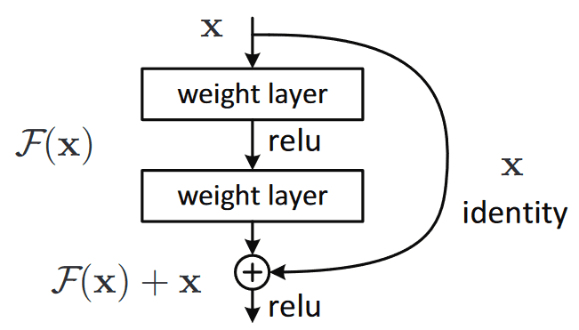Image is taken from Res-Net original paper

Mathematically, we can represent the residual block, and calculate its partial derivative (gradient), given the loss function like this:

\frac{\partial L}{\partial x } = \frac{\partial L}{\partial H} \frac{\partial H}{\partial x} = \frac{\partial L}{\partial H} ( \frac{\partial F}{\partial x} + 1 ) = \frac{\partial L}{\partial H} \frac{\partial F}{\partial x} + \frac{\partial L}{\partial H}

Apart from the vanishing gradients, there is another reason that we commonly use them. For a plethora of tasks (such as semantic segmentation, optical flow estimation , etc.) there is some information that was captured in the initial layers and we would like to allow the later layers to also learn from them. It has been observed that in earlier layers the learned features correspond to lower semantic information that is extracted from the input. If we had not used the skip connection that information would have turned too abstract.

DenseNet: skip connections via concatenation

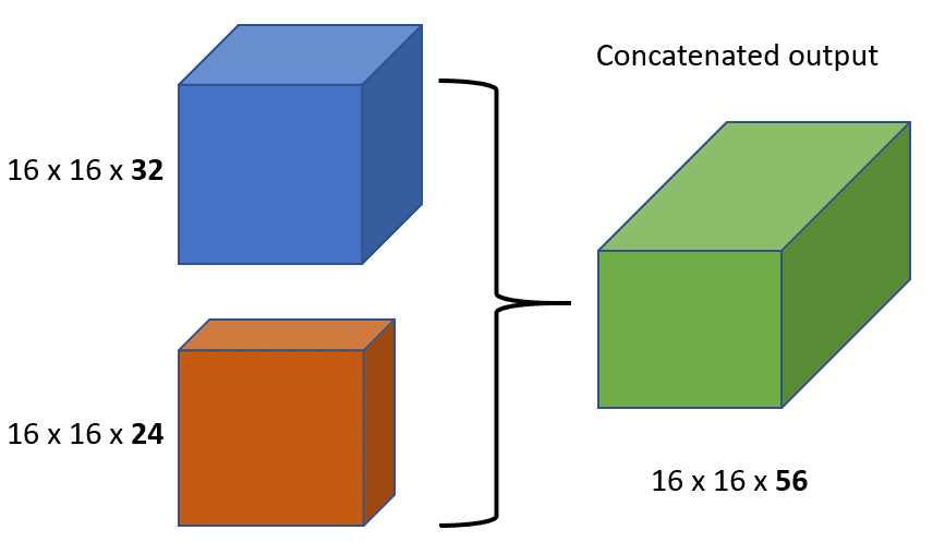
As stated, for many dense prediction problems, there is low-level information shared between the input and output, and it would be desirable to pass this information directly across the net. The alternative way that you can achieve skip connections is by concatenation of previous feature maps. The most famous deep learning architecture is DenseNet. Below you can see an example of feature resusability by concatenation with 5 convolutional layers:

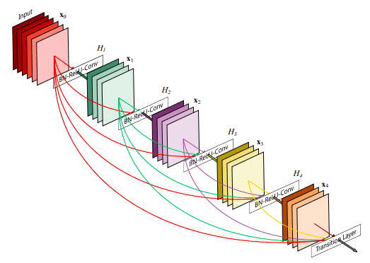Image is taken from DenseNet original paper

This architecture heavily uses feature concatenation so as to ensure maximum information flow between layers in the network. This is achieved by connecting via concatenation all layers directly with each other, as opposed to ResNets. Practically, what you basically do is to concatenate the feature channel dimension. This leads to

a) an enormous amount of feature channels on the last layers of the network,

b) to more compact models, and

c) extreme feature reusability.

Short and Long skip connections in Deep Learning

In more practical terms, you have to be careful when introducing additive skip connections in your deep learning model. The dimensionality has to be the same in addition and also in concatenation apart from the chosen channel dimension. That is the reason why you see that additive skip connections are used in two kinds of setups:

a) short skip connections

b) long skip connections.

Short skip connections are used along with consecutive convolutional layers that do not change the input dimension (see Res-Net), while long skip connections usually exist in encoder-decoder architectures. It is known that the global information (shape of the image and other statistics) resolves what, while local information resolves where (small details in an image patch).

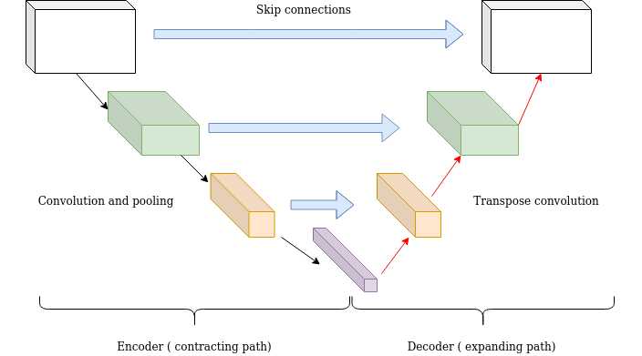
Long skip connections often exist in architectures that are symmetrical, where the spatial dimensionality is reduced in the encoder part and is gradually increased in the decoder part as illustrated below. In the decoder part, one can increase the dimensionality of a feature map via transpose convolutional layers. The transposed convolution operation forms the same connectivity as the normal convolution but in the backward direction.

U-Nets: long skip connections

Mathematically, if we express convolution as a matrix multiplication, then transpose convolution is the reverse order multiplication (BxA instead of AxB). The aforementioned architecture of the encoder-decoder scheme along with long skip connections is often referred as U-shape (Unet). It is utilized for tasks that the prediction has the same spatial dimension as the input such as image segmentation, optical flow estimation, video prediction, etc.

Long skip connections can be formed in a symmetrical manner, as shown in the diagram below:

By introducing skip connections in the encoder-decoded architecture, fine-grained details can be recovered in the prediction. Even though there is no theoretical justification, symmetrical long skip connections work incredibly effectively in dense prediction tasks (medical image segmentation).

Conclusion

To sum up, the motivation behind this type of skip connections is that they have an uninterrupted gradient flow from the first layer to the last layer, which tackles the vanishing gradient problem. Concatenative skip connections enable an alternative way to ensure feature reusability of the same dimensionality from the earlier layers and are widely used.

On the other hand, long skip connections are used to pass features from the encoder path to the decoder path in order to recover spatial information lost during downsampling. Short skip connections appear to stabilize gradient updates in deep architectures. Finally, skip connections enable feature reusability and stabilize training and convergence.

As a final note, encouraging further reading , it has been experimentally validated Li et al 2018 the the loss landscape changes significantly when introducing skip connections, as illustrated below:

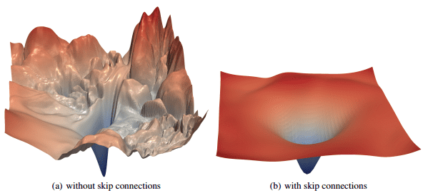Image is taken from this paper

If you need more information about Skip Connections and Convolutional Neural Networks, the Convolutional Neural Network Course online course by Andrew Ng and Coursera is your best option. It is a very comprehensive material with detailed explanations on how the models are applied in real-world applications, and it will cover everything you want. Besides, it has a 4.9/5 rating. That has to mean something.

Cited as:

@article{adaloglou2020skip,
    title   = "Intuitive Explanation of Skip Connections in Deep Learning",
    author  = "Adaloglou, Nikolas",
    journal = "https://theaisummer.com/",
    year    = "2020",
    url     = "https://theaisummer.com/skip-connections/"
  }

References

Çiçek, Ö., Abdulkadir, A., Lienkamp, S. S., Brox, T., & Ronneberger, O. (2016, October). 3D U-Net: learning dense volumetric segmentation from sparse annotation. In International conference on medical image computing and computer-assisted intervention (pp. 424-432). Springer, Cham.
Ronneberger, O., Fischer, P., & Brox, T. (2015, October). U-net: Convolutional networks for biomedical image segmentation. In International Conference on Medical image computing and computer-assisted intervention (pp. 234-241). Springer, Cham.
He, K., Zhang, X., Ren, S., & Sun, J. (2016). Deep residual learning for image recognition. In Proceedings of the IEEE conference on computer vision and pattern recognition (pp. 770-778).
Rumelhart, D. E., Hinton, G. E., & Williams, R. J. (1986). Learning representations by back-propagating errors. nature, 323(6088), 533-536.
Nielsen, M. A. (2015). Neural networks and deep learning (Vol. 2018). San Francisco, CA, USA:: Determination press.
Huang, G., Liu, Z., Van Der Maaten, L., & Weinberger, K. Q. (2017). Densely connected convolutional networks. In Proceedings of the IEEE conference on computer vision and pattern recognition (pp. 4700-4708).
Drozdzal, M., Vorontsov, E., Chartrand, G., Kadoury, S., & Pal, C. (2016). The importance of skip connections in biomedical image segmentation. In Deep Learning and Data Labeling for Medical Applications (pp. 179-187). Springer, Cham.
Li, H., Xu, Z., Taylor, G., Studer, C., & Goldstein, T. (2018). Visualizing the loss landscape of neural nets. In Advances in Neural Information Processing Systems (pp. 6389-6399).

* Disclosure: Please note that some of the links above might be affiliate links, and at no additional cost to you, we will earn a commission if you decide to make a purchase after clicking through.