Spiking Neural Networks: where neuroscience meets artificial intelligence

High energy consumption and the increasing computational cost of Artificial Neural Network (ANN) training ¹ tend to be prohibitive. Furthermore, their difficulty and inability to learn even simple temporal tasks seem to trouble the research community.

Nonetheless, one can observe natural intelligence with minuscule energy consumption, capable of creativity, problem-solving, and multitasking. Biological systems seem to have mastered information processing and response through natural evolution. The need to understand what makes them so effective and adapt these findings led to Spiking Neural Networks (SNNs).

In this article, we will cover both the theory and a simplistic implementation of SNNs in PyTorch.

Information representation: the spike

Biological neuron cells do not behave like the neuron we use in ANNs. But what is it that makes them different?

One major difference is the input and output signals a biological neuron can process. The biological neuron’s output is not a float number to be propagated. Instead, the output is an electric current caused by the movements of ions in the cell. These currents move forward to the connected cells through the synapse. When the propagated current reaches the next cells, it increases their membrane potential, which is a result of the imbalanced concentrations of these ions.

When the membrane potential of a neuron exceeds a certain threshold, the cell emits a spike, i.e. the current to be passed to forward cells ². To this end, using our understanding of typical ANNs, we can map the output of a neuron as a binary value, where 1 represents the spike’s existence in time, and the synapse as the weight that connects two neurons.

One more feature of the biological neurons that arise from this mapping, is asynchronous communication and information processing. Typical ANNs transfer information in sync, wherein in one step, a layer reads an input, computes an output, and feeds it forward. Biological neurons, on the other hand, rely on the temporal dimension. At any moment, they can take an input signal and produce an output, regardless of the behavior of the rest of the neurons.

To sum up, biological neurons have inner dynamics that cause them to change through time. As time passes, they tend to discharge and decrease their membrane potential. Hence, sparse input spikes will not cause a neuron to fire.

To further understand how biological neurons behave , we will look at an example. We will model the neuron using the Leaky Integrate-and-Fire model, one of the simplest models to be used for SNNs.

Leaky Integrate and Fire

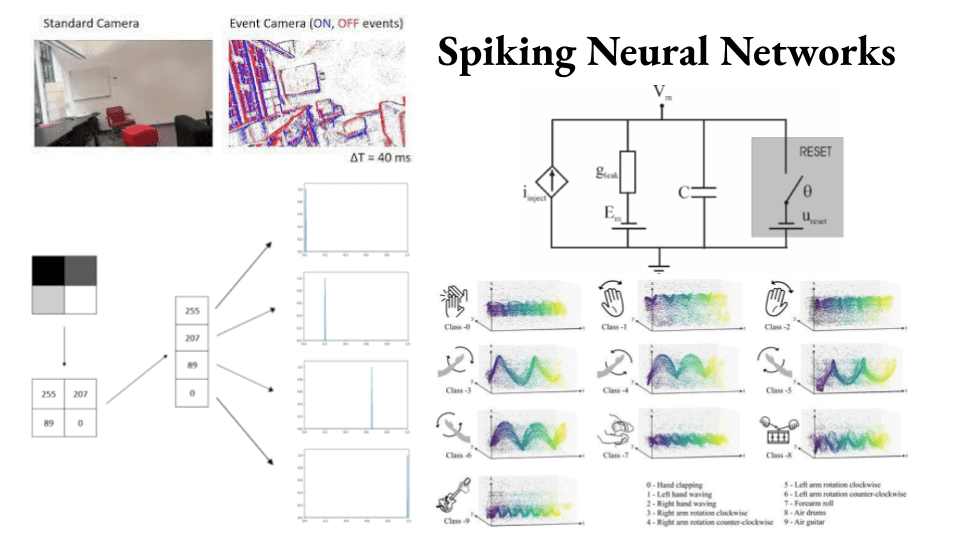
The Leaky Integrate-and-Fire (LIF) model ³ can be represented as a Resistor-Capacitor circuit (RC circuit)⁴, with an input that feeds the circuit with spikes and a threshold switch which causes… well, we will see what it does.

Briefly, the solution of the circuit analysis results in an exponential decay through time with sudden increases of the value of the input.

In more detail, let's set the steady-state voltage at 0. When an input current arrives with the value V, the voltage will increase by V volts. Then, this voltage will start to decay exponentially until a second spike arrives. When an input spike causes the voltage to exceed the threshold (i.e. 1 Volt), then the neuron emits a spike itself and resets to the initial state.

RC circuit. Source: Design of the spiking neuron having learning capabilities based on FPGA circuits)

\tau_{m}\frac{dV_{m}(t)}{dt}=-(V_{m}-E_{m})+\frac{i_{inject}}{g_{leak}}

In this equation, the term $\tau_{m}=C/g_{leak}$ represents a time constant, the so-called membrane time constant, which controls the decay rate of the neuron. $V_{m}$ and $E_{m}$ represent the membrane’s voltage and initial state voltage of the neuron respectively. The input signal is fed through the term $i_{inject}$ .

In the following figure, we see the response of the neuron when an input spike of value 0.8 arrives. The exponential decay can be easily shown, but here we do not exceed the threshold of 1. So the neuron neither does reset its voltage nor emits a spike.

The LIF neuron model allows us to control its dynamics by manipulating its hyperparameters, such as the decay rate or the threshold value. Let’s consider the case where we control the decay rate. An increase in the decay rate would cause the neuron to fire more sparsely in time, or correlate events in time.

In the following figure, we see the input spikes in the temporal dimension. Spikes arrive at the neuron at times 0.075s, 0.125s, 0.2s e.t.c.

Afterward, we observe the response of three neurons. The first neuron has a decay rate of 0.05 (1/200) and the input spikes have a value of 0.5 (the weight of the synapse is 0.5). Consequently, the neuron is not reaching the threshold value, since its voltage drops quickly so the neuron does not emit any spikes.

Lowering both the decay rate to 0.025 (1/400) and the synapse weight to 0.35 results in the neuron firing once at time 0.635s.

Nonetheless, we may want the neuron to spike at “packed” events, as in our example, at the interval (0, 0.2) and (0.6, 0.8). We see that we achieve the desired result by adjusting the synapse weight back to 0.5.

This inner dynamic of the neuron and the asynchronous behavior of the network, has been the key to SNNs. Noteworthy results have been obtained in difficult spatiotemporal tasks ⁵, ⁶ and research in neuromorphic hardware. The latter implements SNNs with low energy consumption ⁷.

One might ask how complex data (such as images) is fed to the network. Image datasets like MNIST contain images with a single set of values for each pixel (RGB, Gray-scale etc), while, as we have discussed, SNNs can handle and process sequences of spikes, the so-called spiketrain.

A spiketrain is a sequence of spikes over a time window.

But how can you transform inputs into spiketrains? Two methods can be used:

encoding algorithms and,
event cameras (for visual processing).

Information encoding

Information encoding is the process of getting an input signal, and converting it into spiketrains.

One such simple encoding method is the Poisson encoding ⁸, where a value of the signal to be given as an input to a neuron, is normalized between the minimum and the maximum value. The normalized value represents a probability of $r$ . Over a time window $T$ and a small timestep $dt$ , the resulting spiketrain of the encoded signal, at each timestep $dt$ , has probability $rdt$ of containing a spike. In this way, the higher the probability $r$ , the more spikes the resulting spiketrain will have. Thus the information will be encoded more accurately.

Images to spiketrains

Let's see an example. Imagine a grayscale image of size 32x32 pixel. The value of the pixel at position (1,1) is 32. Normalizing the value we get $r=32/256 => r = 0.125$ . Over the time window of 1 second and $dt = 0.001$ seconds, the resulting spiketrain will have about $r*T/dt = 125$ spikes, with the total number of them following a Gaussian distribution. At each timestep 0.001, we expect a probability of 0.125 of finding a spike.

P(1\:spike\:during\:dt) \approx rdt

P(n\:spikes\:during\:\Delta t) = e^{-r\Delta t}\frac{(r\Delta t)^n}{n!}

This method shows high biological plausibility since human vision seems to store information the same way for the first layer of neurons. However, this disregards the information encoded at the exact timing of the spike.

One can easily realize this, since two identical values may result in a different spiketrain.

Rank Order Coding and Population Order Coding

To alleviate this problem, a wide variety of algorithms have been proposed, such as Rank Order Coding (ROC) ⁹ or Population Order Coding (POC) ¹⁰. ROC encodes the information in the order the spikes arrive, over a given time window, with the first spike meaning the highest value of the signal. This results in losses in information. POC solves this problem by encoding a single value in multiple neurons that use receptive fields that cover all the possible values.

Let us see two encoding-to-spikes methods, one rate-based (Poisson Encoder) and one temporal-based (ROC-like). Have a look at the following figure.

Poisson encoder

Trying to process this 2 by 2 grayscale image, we realize that it is stored as 4 integers in the range of 0 (for white) to 255 (for brack). In ANNs this set of numbers is the input vector that is fed to the network. We want to transform it into spiketrains in a given time window; for example 1ms with $dt$ of 0.02ms. This results in 50 discrete timesteps.

The Poisson encoding method will produce a proportional number of spikes for the given time window as shown below. The value of 255 will be packed with spikes, the value of 207 will produce less and so it goes for the rest.

On the other hand, the temporal method will produce only one spike for each value but the information is encoded in the timing of this spike, where the highest values produce an early spike compared to lower ones.

Temporal-based encoder

Both of them have their pros and cons ¹¹. Even a look into nature and how biological brains handle the information is enough to understand that both types or a mix of them are used ¹².

The choice of the encoding algorithms affects the result of the neuron’s output and the behavior of the network in general. Moreover, not all developed learning schemes can be applied to every encoding scheme. Some learning methods rely on the information coded in the exact timing of the spike and so rate encoding algorithms like the Poisson encoding algorithms will not work, and vice versa.

Many more algorithms have been developed such as Temporal Contrast ¹³, HSA ¹⁴, BSA ¹⁵ that can provide a wide variety of choices.

On the other side, event cameras, most known as Dynamic Vision Sensors (DVS), overcome the whole encoding process, by recording input, such as video, directly into spiketrains.

Dynamic Vision Sensors (DVS)

In video recording, typical cameras map a value at each pixel for every timestep (frame).

DVS ¹⁶, on the contrary, focuses on the brightness intensity differences. When the brightness changes enough over two consecutive timesteps, the camera produces an “event”.

This event stores: a) the information about the occurrence of the spike (simply, that a spike is generated), b) the pixel that produces the spike in the form of its spatial coordinates $X$ , $Y$ , c) the timestamp that the event occurs and d) the polarity.

Polarity denotes whether the threshold was over exceeded or under exceeded. So when the intensity increases over the threshold, the polarity will be positive. On the other hand, when it decreases over the (negative) threshold, it will be negative. The polarity storage requires the existence of “negative” spikes but it also adds to the information for the network, since it can use this attribute to extract more meaningful results.

\Delta L(x_{k},t_{k}) = L(x_{k},t_{k})-(x_{k},t_{k}-\Delta t_{k})

\Delta L(x_{k},t_{k}) = p_{k}C

Sandard camera vs DVS. Source: Event Cameras

This picture shows the data produced by a dynamic vision sensor. On the left, we see the image from a standard camera. On the right, we see the same picture taken by a DVS. Here, we see the aforementioned positive and negative spikes produced by the sensor. Again, DVS takes spatiotemporal data. DVS collect and compare luminance differences through time. The picture above does not make this clear.

In the following figure, we see both the temporal and spatial components of the resulting recording. The yellow spikes denote early produced spikes, while the purple ones, late produced spikes. Note that this image does not contain polarity information.

Source: Space-time event clouds for gesture recognition: From RGB cameras to event cameras

One can argue that the data produced by such sensors lag behind in information contained compared to standard cameras. Importantly though, DVS:

use only a fraction of the energy consumed by typical vision recorders,
can operate to frequencies up to 1MHz, and
do not blur the resulting image or video ¹⁷.

This makes them very appealing to the research community and a possible candidate for robotic systems with limited energy sources.

Training the SNN

You have seen how to model the neuron for our network, studied its response, and analyzed the encoding methods to get our desired input. Now comes the most important process: the training of the network. How does the human brain learn, and what does it even mean?

Learning is the process of changing the weight that connects neurons in a desirable way. Biological neurons, though, use synapses to communicate information. The weight change is equivalent to the connection strength of the synapse, which can be altered through time with processes that cause synaptic plasticity. Synaptic plasticity is the ability of the synapse to change its strength.

Synaptic Time Dependent Plasticity (STDP)

“Neurons that fire together, wire together”. This phrase describes the well-known Hebbian learning and the Synaptic Time Dependent Plasticity (STDP) ¹⁸ learning method that we will discuss. STDP is an unsupervised method that is based on the following principle.

A neuron adapts its pre-synaptic input spike (the input weight of a previous neuron) to match the timing of an input spike with the output spike.

A mathematical expression will help us understand.

\Delta w_{j}=\sum_{f=1}^N\sum_{n=1}^N W(t_{i}^n-t_{j}^f)

Source: Spike-Timing-Dependent-Plasticity (STDP) models or how to understand memory.

Let's think of an input weight $w_1$ . If the spike that comes from $w_1$ arrives after the neuron has emitted the spike, the weight decreases because the input spike has no effect on the output one.

On the other hand, a spike arriving before the fire of a neuron strongly affects the timing of the neuron’s spike, and so its weight increases to temporally connect the two neurons through this synapse (weight $w_1$ ).

Due to this process, patterns emerge in the connections of the neurons, and it has been shown that learning is achieved.

But STDP is not the only learning method.

SpikeProp

SpikeProp ¹⁹ is one of the first learning methods to be used. It can be thought of as a supervised STDP learning method.

The core principle is the same: it changes the synapse weight based on the spike timing. The difference with STDP is that while STDP measures the difference in presynaptic and postsynaptic spike timing, here we focus only on the resulting spikes of the neuron (postsynaptic) and their timing.

Since it is a supervised learning method, we need a target value, which is the desired firing time of the output spike. The loss function and the proportional weight change of the synapse are dependent on the difference in the resulting spike timing and the desired spike timing.

In other words, we try to change the input synapse weight in such a way that the timing of the output spike matches the desired timing for the resulting spike.

If we take a look at the equation of the loss function, we notice its similarity with the STDP weight update rule.

E=1/2\sum_{j\in J}(t_{j}^a-t_{j}^d)^2

The fact that we consider the difference of the output with the desired spike timing, allows us to: a) create classes to classify data and b) use the loss function with a backpropagation-like rule to update the input weight of the neurons.

\Delta w_{ij}^k=-\eta \frac{\partial E}{\partial w_{ij}^k}

\Delta w_{ij}^k=-\eta y_{i}^k (t_{j}^a) \delta_{j}

The term $\delta_{j}$ is a key-term for the weight update and is equal to the following equation:

\delta_{j} = \frac { t_{j}^d-t_{j}^a} {\sum_{i \in \Gamma_{j} } \sum_{l} w_{ij}^l(\partial y_{i}^l(t_{j}^a) / \partial t_{j}^a)}

The adaptation of the delta term can give us a backpropagation rule for SpikeProp with multiple layers.

This method illustrates the power of SNNs. With SpikeProp we can code a single neuron to classify multiple classes of a given problem. For example, if we set the desired output timing for the first class at 50 ms, for the second at 75ms, a single neuron can distinguish multiple classes. The drawback of this is that the neuron will only have access to the first 50ms of information to decide if an input belongs to the first class.

Implementation in Python

The steadily increasing interest in Spiking Neural Networks has led to many attempts in developing SNN libraries for Python. Only to mention a few, Norse, PySNN and snnTorch have done an amazing job in simplifying the process of deep learning with the use of spiking neural networks. Note that they also contain complete documentation and tutorials.

Now, let’s see how we could create our own classifier for the well-known MNIST dataset. We will use the snnTorch library by Jason Eshraghian ²⁰ for our purpose since it makes it easy to understand the network’s architecture. SnnTorch can be thought of as a library extending the PyTorch library.

If you want to execute the code yourself, you can do so from our Google colab notebook.

Let’s install snntorch using pip install and import the necessary libraries

$ pip install snntorch

import snntorch as snn
import torch

First, we have to load our dataset. The MNIST dataset, as you may know, is static. So, we have to encode the data into spikes. The code below uses the rate encoding method to produce the desired result with the spikegen.rate() function, although both latency (temporal) and delta modulation encoding methods have been implemented. You are free to try using the functions spikegen.latency() and spikegen.delta() to see the differences.

We use torchvision for the transformation and loading of the data.

from torchvision import datasets, transforms
from snntorch import utils
from torch.utils.data import DataLoader
from snntorch import spikegen

# Training Parameters
batch_size=128
data_path='/data/mnist'
num_classes = 10  # MNIST has 10 output classes

# Torch Variables
dtype = torch.float

# Define a transform
transform = transforms.Compose([
            transforms.Resize((28,28)),
            transforms.Grayscale(),
            transforms.ToTensor(),
            transforms.Normalize((0,), (1,))])

mnist_train = datasets.MNIST(data_path, train=True, download=True, transform=transform)
mnist_test = datasets.MNIST(data_path, train=False, download=True, transform=transform)

train_loader = DataLoader(mnist_train, batch_size=batch_size, shuffle=True)
test_loader = DataLoader(mnist_test, batch_size=batch_size, shuffle=True)

num_steps = 100

# Iterate through minibatches
data = iter(train_loader)
data_it, targets_it = next(data)

# Spiking Data
spike_data = spikegen.rate(data_it, num_steps=num_steps)

The num_steps variable sets the duration of the spiketrain from the static input image. If we increase the number of steps, we see that the average number of spikes tends to the value of the pixel. You may try to run the code below with different values of _num_steps _to see if the expected behavior follows.

num_steps = 1000

# Iterate through minibatches
data = iter(train_loader)
data_it, targets_it = next(data)

# Spiking Data
spike_data = spikegen.rate(data_it, num_steps=num_steps)

img = 13
x, y = 12, 12
print(float(sum(spike_data[:,img,0,x,y])/num_steps), data_it[img,0,x,y])

Now, it’s time to create the neuron. The simplest one to code is the Leaky Integrate and Fire neuron model (LIF). The code is as simple as shown below:

def leaky_integrate_and_fire(mem, x, w, beta, threshold=1):
  spk = (mem > threshold) # if membrane exceeds threshold, spk=1, else, 0
  mem = beta * mem + w*x - spk*threshold
  return spk, mem

The mem variable holds the inner state, the membrane potential of the neuron, while a spike is produced when the potential exceeds the threshold. We could implement and run a simulation of the neuron by hand (code each step of the way as it is done in the snntorch tutorial). However, the neuron’s instance can be set with one line of code implemented by snntorch:

lif1 = snn.Leaky(beta=0.8)

To develop a layer of LIF neurons, the library uses the above command with the addition of a typical torch Linear or Convolutional Layer. With the code below, we set the architecture of the network:

# layer parameters
num_inputs = 784
num_hidden = 1000
num_outputs = 10
beta = 0.99

# initialize layers
fc1 = nn.Linear(num_inputs, num_hidden)
lif1 = snn.Leaky(beta=beta)
fc2 = nn.Linear(num_hidden, num_outputs)
lif2 = snn.Leaky(beta=beta)

We now have enough to run forward iterations with our network. However, this is not the way to go here. If we continue like that, we lose the wide variety that PyTorch offers, such as built-in optimizers and methods.

Following the PyTorch design pattern, we code a class to implement our network with the forward function to produce the resulting spiketrains for each of the layers. The function _self.lif.init_leaky()_ initiates the parameters for the layer.

import torch.nn as nn

# Network Architecture
num_inputs = 28*28
num_hidden = 1000
num_outputs = 10

# Temporal Dynamics
num_steps = 25
beta = 0.95

# Define Network
class Net(nn.Module):

    def __init__(self):
        super().__init__()

        # Initialize layers
        self.fc1 = nn.Linear(num_inputs, num_hidden)
        self.lif1 = snn.Leaky(beta=beta)
        self.fc2 = nn.Linear(num_hidden, num_outputs)
        self.lif2 = snn.Leaky(beta=beta)

    def forward(self, x):

        # Initialize hidden states at t=0
        mem1 = self.lif1.init_leaky()
        mem2 = self.lif2.init_leaky()

        # Record the final layer
        spk2_rec = []
        mem2_rec = []

        for step in range(num_steps):
            cur1 = self.fc1(x)
            spk1, mem1 = self.lif1(cur1, mem1)
            cur2 = self.fc2(spk1)
            spk2, mem2 = self.lif2(cur2, mem2)
            spk2_rec.append(spk2)
            mem2_rec.append(mem2)

        return torch.stack(spk2_rec, dim=0), torch.stack(mem2_rec, dim=0)

# Load the network onto CUDA if available
device = torch.device("cuda") if torch.cuda.is_available() else torch.device("cpu")

net = Net().to(device)

In order to train the network, we will use the backpropagation through time method (BPTT). This method is basically backpropagation for each timestep of the spiketrain. This means that we can use the Adam optimizer to train our network. We set our loss function and the optimizer:

loss = nn.CrossEntropyLoss()
optimizer = torch.optim.Adam(net.parameters(), lr=5e-4, betas=(0.9, 0.999))

Now, all that is left is the training loop of our network. The implementation of this loop is similar to other ANNs with the difference in the storage of the neuron dynamics during the runs. Let’s code the training iteration for one epoch:

num_epochs = 1
loss_hist = []
test_loss_hist = []
counter = 0

# Outer training loop
for epoch in range(num_epochs):
    train_batch = iter(train_loader)

    # Minibatch training loop
    for data, targets in train_batch:
        data = data.to(device)
        targets = targets.to(device)

        # forward pass
        net.train()
        spk_rec, mem_rec = net(data.view(batch_size, -1))

        # initialize the loss & sum over time
        loss_val = torch.zeros((1), dtype=dtype, device=device)
        for step in range(num_steps):
            loss_val += loss(mem_rec[step], targets)

        # Gradient calculation + weight update
        optimizer.zero_grad()
        loss_val.backward()
        optimizer.step()

        # Store loss history for future plotting
        loss_hist.append(loss_val.item())

        # Test set
        with torch.no_grad():
            net.eval()  
            test_data, test_targets = next(iter(test_loader))
            test_data = test_data.to(device)
            test_targets = test_targets.to(device)

            # Test set forward pass
            test_spk, test_mem = net(test_data.view(batch_size, -1))

            # Test set loss
            test_loss = torch.zeros((1), dtype=dtype, device=device)

            for step in range(num_steps):
                test_loss += loss(test_mem[step], test_targets)

            test_loss_hist.append(test_loss.item())

            # Print test loss
            if counter % 50 == 0:
                print(“Test loss: “, float(test_loss))

            counter += 1

And it is done! As the network is training, we see the test loss value decrease, indicating the ability of the network to be trained in the given dataset.

We have to mention that the above setup of the network does not need the input to be passed as spiketrains, rather it handles numerical values for each pixel of the MNIST dataset.

Conclusion and further reading

In this article, we have only scratched the surface of the algorithms for SNN training. The property of STDP can be implemented in more complex setups even for supervised learning algorithms, while SpikeProp does not seem like a suitable choice for multi-perceptron layers.

A wide variety of algorithms, based on biological processes or borrowing ideas from ANN learning algorithms, have been implemented. Such interesting ideas are the common BackPropagation Through Time (BPTT) ²¹, its recent successor E-prop ²², the local learning-based DECOLLE ²³, and the kernel-based SuperSpike ²⁴ algorithms.

By now, I hope you have gotten the core idea of the SNNs. What the ‘spike’ is for the SNN and how it is encoded. How the ‘temporal dynamics’ of the neurons affect the behavior of the network. We strongly suggest studying the well-documented tutorials of snntorch and experimenting with as many of the hyperparameters as you can, to acquire a better understanding of what happens in the inner structure.

Cite as

@article{korakovounis2021spiking,
  title   = "Spiking Neural Networks: where neuroscience meets artificial intelligence",
  author  = "Korakovounis, Dimitrios",
  journal = "https://theaisummer.com/",
  year    = "2021",
  url     = "https://theaisummer.com/spiking-neural-networks/"
}

References

Neil C. Thompson, Kristjan Greenewald, Keeheon Lee, Gabriel F. Manso. Deep learning computational cost, 2021 ↩
Wikipedia: Action potential ↩
Nicolas Brunel, Mark C.W. Van Rossum, Quantitative investigations of electrical nerve excitation treated as polarization. Biological Cybernetics, 97:341–349, 2007.↩
Samuel J. Ling, Jeff Sanny, William Moebs, Daryl Janzen, Introduction to Electricity, Magnetism, and Circuits. Chapter 6.5: RC Circuits, ↩
Leslie S Smith, Dagmar S Fraser. Sound feature detection using leaky integrate-and-fire neurons, 2004↩
Effrosyni Doutsi, Lionel Fillatre, Marc Antonini, Panagiotis Tsakalides. Dynamic Image Quantization Using Leaky Integrate-and-Fire Neurons. IEEE Transactions on Image Processing, 30:4305–4315, 2021↩
Junxiu Liu, Yongchuang Huang, Yuling Luo, Jim Harkin, Liam McDaid. Bio-inspired fault detection circuits based on synapse and spiking neuron models. Neurocomputing, 331:473–482, 2019↩
David Heeger, Poisson Model of Spike Generation, 2000↩
Simon Thorpe, Jacques Gautrais, Rank Order Coding, 1998.↩
Nikola K Kasabov. Time-Space, Spiking Neural Networks and Brain-Inspired Artificial Intelligence, 2019↩
Wikipedia: Neural coding ↩
John Huxter, Neil Burgess, John O’Keefe. Independent rate and temporal coding in hippocampal pyramidal cells. Nature, 425:824–828, 2003↩
Balint Petro, Nikola Kasabov, Rita M. Kiss. Selection and Optimization of Temporal Spike Encoding Methods for Spiking Neural Networks. IEEE Transactions on Neural Networks and Learning Systems, 31:358–370, 2020↩
Felix Gers, Norberto Eiji Nawa, Michael Hough, Hugo De Garis, Michael Korkin. SPIKER: Analog Waveform to Digital Spiketrain Conversion in ATR's Artificial Brain (CAM-Brain) Project, Digital Microbiology Lab View project CoDi-A CELLULAR AUTOMATA BASED NEURAL NET MODEL View project Michael Korkin Independent Researcher, 1999.↩
Benjamin Schrauwen, Jan Van Campenhout, BSA, a Fast and Accurate SpikeTrain Encoding Scheme. Vol. 4, p. 2825–2830, 2003↩
Wikipedia: Event camera ↩
Min Liu, Tobi Delbruck, Block-Matching Optical Flow for Dynamic Vision Sensors: Algorithm and FPGA Implementation, 2017 IEEE International Symposium on Circuits and Systems (ISCAS), 2017↩
H. Markram, W. Gerstner P. J. Sjöström, Spike-Timing-Dependent Plasticity: A Comprehensive Overview, Frontiers in Synaptic Neuroscience, 4, 2012.↩
Sander M Bohte, Joost N Kok, Han La Poutrã. Error-backpropagation in temporally encoded networks of spiking neurons, 2002↩
Jason K. Eshraghian, Max Ward, Emre Neftci, Xinxin Wang, Gregor Lenz, Girish Dwivedi, Mohammed Bennamoun, Doo Seok Jeong, Wei D. Lu, Training Spiking Neural Networks Using Lessons From Deep Learning, September 2021↩
Yujie Wu, Lei Deng, Guoqi Li, Jun Zhu, Luping Shi, Spatio-temporal backpropagation for training high-performance spiking neural networks, Frontiers in Neuroscience, 12, 2018↩
Guillaume Bellec, Franz Scherr, Anand Subramoney, Elias Hajek, Darjan Salaj, Ro-bert Legenstein, Wolfgang Maass, A solution to the learning dilemma for recurrent networks of spiking neurons, Nature Communications, 11, 2020.↩
Jacques Kaiser, Hesham Mostafa, Emre Neftci, Synaptic Plasticity Dynamics for Deep Continuous Local Learning (DECOLLE), Frontiers in Neuroscience, 14, 2020↩
Friedemann Zenke, Surya Ganguli, SuperSpike: Supervised learning in multi-layer spiking neural networks, October 2017↩

* Disclosure: Please note that some of the links above might be affiliate links, and at no additional cost to you, we will earn a commission if you decide to make a purchase after clicking through.