Data preprocessing for deep learning: How to build an efficient big data pipeline

In this article, we explore the topic of big data processing for machine learning applications. Building an efficient data pipeline is an essential part of developing a deep learning product and something that should not be taken lightly. As I‘m pretty sure you know by now, machine learning is completely useless without the right data. And by the right data, we mean data from the correct sources and in the right format.

But what is a data pipeline? And when do we characterize it as efficient?

Generally speaking, data prepossessing consists of two steps: Data engineering and feature engineering.

Data engineering is the process of converting raw data into prepared data, which can be used by the ML model.
Feature engineering creates the features expected by the model.

When we deal with a small number of data points, building a pipeline is usually straightforward. But that’s almost never the case with Deep Learning. Here we play with very very large datasets (I’m talking about GBs or even TBs in some cases). And manipulating those is definitely not a piece of cake. But dealing with difficult software challenges is what this article series is all about. If you do not know what I’m talking about here is a brief reminder:

This article is the 5th part of the Deep Learning in Production series. In the series, we are starting from a simple experimental jupyter notebook with a neural network that performs image segmentation and we write our way towards converting it in production-ready highly-optimized code and deploy it to a production environment serving millions of users. If you missed that, you can start from the first article.

Back to data processing. Where were we? Oooh yeah. So how do we build efficient big data pipelines to feed the data into the machine learning model? Let’s start with the fundamentals.

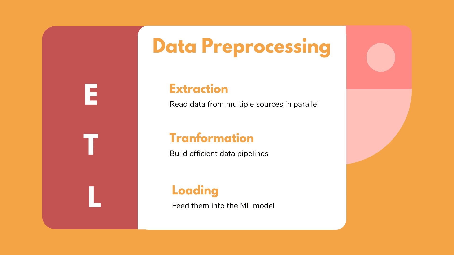
ETL: Extract, Transform, Load

In the wonderful world of databases, there is this notion called ETL. As you can see in the headline ETL is an acronym of Extract, Transform, Load. These are the 3 building blocks of most data pipelines.

Extraction involves the process of extracting the data from multiple homogeneous or heterogeneous sources.
Transformation refers to data cleansing and manipulation in order to convert them into a proper format.
Loading is the injection of the transformed data into the memory of the processing units that will handle the training (whether this is CPUs, GPUs or even TPUs)

When we combine these 3 steps, we get the notorious data pipeline. However, there is a caveat here. It’s not enough to build the sequence of necessary steps. It’s equally important to make them fast. Speed and performance are key parts of building a data pipeline.

Why? Imagine that each training epoch of our model, it’s taking 10 minutes to complete. What happens if ETL of the segment of the required data can’t be finished in less than 15 minutes? The training will remain idle for 5 minutes. And you may say fine, it’s offline, who cares? But when the model goes online, what happens if the processing of a datapoint takes 2 minutes? The user will have to wait for 2 minutes plus the inference time. Let me tell you that 2 minutes in browser response time is simply unacceptable for good user experience.

If you are still with me, let’s see how things work in practice. Before we dive into the details, let’s see some of the problems we want to address when constructing an input pipeline. Because it’s not just speed (if only it was). We also care about throughput, latency, ease of implementation and maintenance. In more details, we might need to solve problems such as :

Data might not fit into memory.
Data might not even fit into the local storage.
Data might come from multiple sources.
Utilize hardware as efficiently as possible both in terms of resources and idle time.
Make processing fast so it can keep up with the accelerator’s speed.
The result of the pipeline should be deterministic (or not).
Being able to define our own specific transformations.
Being able to visualize the process.

And many more. I will try to make things as easy as possible but it’s gonna be tricky. For each part of the pipeline, I will explain some basic concepts, the problem we address and then I will present a few lines of code (yes thanks to Tensorflow and the tf.data module, input pipelines are just a few lines of code). Also, we will use the same dataset that comes with the original notebook we’ve used so far, which is a collection of pet images from the Visual Geometry Group of Oxford University. Let’s get right into it.

Source: http://www.robots.ox.ac.uk/~vgg/data/pets/

Data Reading

Data reading or extracting is the step in which we get the data from the data source and convert them from the format they are stored into our desired one. You may wonder where the difficulty is. We can just run a “pandas.read_csv()”. Well not quite. In the research phase of machine learning, we are used to having all the data in our local disk and playing with them. But in a production environment, the data might be stored in a database (like MySQL or MongoDB), or in an object storage cloud service (like AWS S3 or Google cloud storage), or in a data warehouse (like Amazon Redshift or Google BigQuery) or of course in a simple storage unit locally. And each storage option has its own set of rules on how to extract and parse data.

Loading from multiple sources

That’s why we need to be able to consolidate and combine all these different sources into a single entity that can be passed into the next step of the pipeline. And of course, each source has a specific format to store them, so we need a way to decode it as well. Here is a boilerplate code that uses tf.data (the standard data manipulation library of tf)

files = tf.data.Dataset.list_files(file_pattern)
dataset = tf.data.TFRecordDataset(files)

As you see, we define a list of files based on a pattern and then we construct a TFRecordDataset from those files. For example in the case that our data are on AWS s3, we might have something like that:

filenames = ["s3://bucketname/path/to/file1.tfrecord",
             "s3://bucketname/path/to/file2.tfrecord"]
dataset = tf.data.TFRecordDataset(filenames)

But in our case with the pet images can we simply do this?

dataset = tf.data.TFRecordDataset("http://www.robots.ox.ac.uk/~vgg/data/pets/data/images.tar.gz")

Unfortunately no. You see, the data should be in a format and in a source supported by tensorflow. What we want to do here is to manually download, unzip and convert the raw images into tf.Records or another compatible with Tensorflow format. Luckily we can use the tensorflow datasets library (tf.tdfs) for that, which wraps all this functionality and returns a ready to use tf.Dataset.

import tensorflow_datasets as tfds

tfds.load("oxford_iiit_pet:3.*.*", with_info=True)

Or more precisely in our code:

@staticmethod
def load_data(data_config):
    """Loads dataset from path"""
    return tfds.load(data_config.path, with_info=data_config.load_with_info)

But for unsupported datasets, I’m afraid that we have to do that ourselves and create a custom data loader. In the case of BigQuery for example, something like this is a good way to go.

That’s why good knowledge of our data source intricacies is almost always necessary.

Btw (by the way), there is this excellent library called TensorFlow I/O to help us deal with more data formats (it even supports DICOM!)

Are you discouraged already? Don’t be. Creating data loaders is an essential part of being a Machine Learning Engineer. For anyone who is curious on how to build an efficient data loader for an unsupported data source, you can take a peek under the hood on how tensorflow datasets library handles our pet dataset internally.

Parallel data extraction

In cases where data are stored remotely, loading them can become a bottleneck in the pipeline since it can significantly increase the latency and lower our throughput. The time that takes for the data to be extracted from the source and travel into our system is an important factor to take into consideration. What can we do to tackle this bottleneck?

The answer that comes first to mind is parallelization. Since we haven’t touched upon parallel processing so far in the series, let’s give a quick definition:

Parallel processing is a type of computation in which many calculations or the execution of processes are carried out simultaneously.

Modern computing systems include multiple CPU cores, so why not take advantage of all of them (remember efficient hardware utilization?). For example, my laptop has 4 cores. Wouldn’t it be reasonable to assign each core to a different data point and load four of them at the same time? Luckily it is as easy as this:

tf.data.Dataset.list_files(file_pattern)
tf.data.interleave(TFRecordDataset,num_calls=4)

The “interleave()” function will load many data points concurrently and interleave the results so we don’t have to wait for each one of them to be loaded.

Because parallel processing is a highly complicated topic, let’s talk about it more extensively later in the series. For now, all you need to remember is that we can extract many data at the same time utilizing our system resources efficiently. Before the introduction of parallelization the processing flow was something like this:

Open connection ->  read datapoint 1 -> continue -> read datapoint 2 -> continue

But now it is something like this

Open connection -> read datapoint 1 -> continue ->
        -> read datapoint 2 -> continue ->
        -> read datapoint 3 -> continue ->
            -> read datapoint 4 -> continue ->

Data Processing

Well well where are we? We loaded our data in parallel from all the sources and now we are ready to apply some transformations into them. In this step, we are running the most computationally intense functions such as image manipulation, data decoding and literally anything you can code (or find a ready solution for). In the image segmentation example that we are using, this will simply be resizing our images, flip a portion of them to introduce variance in our dataset, and finally normalize them. Although let me introduce another new concept before that, starting from functional programming

Functional programming is a programming paradigm in which we build software by stacking pure functions, avoiding to share state between them and using immutable data. In functional programming, the logic and data flows through functions, inspired by the mathematics

Does that make sense? I’m sure it doesn’t. Let’s give an example.

df.rename(columns={"titanic_survivors": "survivors"})\
  .query("survivors_age > 14 and survivors_gender == "female"")\
  .sort_values("survivors_age", ascending=False)\

Does that seem familiar? It’s pure pandas code. Notice how we chained the methods so each function is called after the previous one. Also notice that we don’t share information between functions and that the original dataset flows throughout the chain. That way we don’t need to have for-loops, or reassign variables over and over or create a new dataframe every time we apply a new transformation. Plus, it is so freaking easy to parallelize this code. Remember the trick above in the interleave function where we add a num_calls argument? Well, the reason we are able to do that so effortlessly is functional programming.

In overly simplified terms, that’s functional programming. I highly encourage you to check out the link on the end for more information. Always keep in mind that no one expects you to understand functional programming from one paragraph. But that’s our intention here in AI Summer: to give the motivation to learn new things and become a well-rounded engineer.

But why do we care? Functional programming supports many different functions such as “filter()”, “sort()” and more. But the most important one is called “map()”. With “map()” we can apply whatever (almost) function we may think of.

Map is a special function that applies a function to each element of a collection. Instead of writing a for-loop and iterating over all elements, we can simply map all the collection’s elements to the result of the user-defined function. And of course it follows the functional paradigm. Actually let’s look at a simple example to make that more clear.

Imagine that we have a list [1,2,3,4] and we want to add 1 to each element and produce a new array with values [2,3,4,5]. In normal python code we have :

m_list = [1,2,3,4]

for i in m_list:
    m[i] = m[i] +1

But in functional programming we can do:

m_list = list( map( lambda i: i+1, m_list) )

And the result is the same. What’s the advantage? It’s much simpler, it improves maintainability, we can define extremely complex functions easily, it provides modularity and is shorter. Plus it makes parallelization so much easier. Try to parallelize the above for-loop. I dare you.

Back to data pipelines. In the segmentation example we can do something like below.

So far in the code from previous articles we have a preprocessing function that resizes, randomly flips and normalize the images

@staticmethod
def _preprocess_train(datapoint, image_size):
    """ Loads and preprocess  a single training image """
    input_image = tf.image.resize(datapoint['image'], (image_size, image_size))
    input_mask = tf.image.resize(datapoint['segmentation_mask'], (image_size, image_size))

    if tf.random.uniform(()) > 0.5:
        input_image = tf.image.flip_left_right(input_image)
        input_mask = tf.image.flip_left_right(input_mask)

    input_image, input_mask = DataLoader._normalize(input_image, input_mask)

    return input_image, input_mask

We can simply add the preprocessing step to the data pipeline using “map()” and lambda functions. The result is:

@staticmethod
def preprocess_data(dataset, batch_size, buffer_size,image_size):
    """ Preprocess and splits into training and test"""
    train = dataset['train'].map(lambda image: DataLoader._preprocess_train(image,image_size), num_parallel_calls=tf.data.experimental.AUTOTUNE)
    train_dataset = train.shuffle(buffer_size)

    test = dataset['test'].map(lambda image: DataLoader._preprocess_test(image, image_size))
    test_dataset = test.shuffle(buffer_size)

    return train_dataset, test_dataset

As you can see, we have two different pipelines. One for the train dataset and one for the test dataset. See how we first apply the “map()” function and sequentially the “shuffle()”. The map function will apply the “_preprocess_train“ in every single datapoint. And once the preprocessing finished it will shuffle the dataset. That’s functional programming babe. No share of objects between functions, no mutability of objects, no unnecessary side effects. We just declare our desired functionality and that’s it. Again I’m sure some of you don’t understand all the terms and that’s fine. The key thing is to understand the high-level concept.

Notice also the “num_parallel_calls” argument. Yup, we will run the function in parallel. And thanks to TensorFlow’s built-in autotuning, we don’t even have to worry about setting the number of calls. It will figure it out by itself, based. How cool is that?

Finally on the Unet class the whole pipeline looks like this:

def load_data(self):
    """Loads and Preprocess data """
    LOG.info(f'Loading {self.config.data.path} dataset...')
    self.dataset, self.info = DataLoader().load_data(self.config.data)
    self.train_dataset, self.test_dataset = DataLoader.preprocess_data(self.dataset, self.batch_size, self.buffer_size, self.image_size)
    self._set_training_parameters()

Not that bad huh? For the full code, you can visit our GitHub repo

For completion’s sake, we also need to mention that besides “map()”, tf.data also supports many other useful functions such as:

filter() : filtering dataset based on condition
shuffle(): randomly shuffle dataset
skip(): remove elements from the pipeline
concatenate(): combines 2 or more datasets
cardinality(): returns the number of elements in the dataset

And of course it contains some extremely powerful functions like “batch()”, “prefetch()”, “cache()”, “reduce()”, which are the topic of the next in line article. The original plan was to have them here as well but it will surely compromise the readability of this article and it will definitely give you a headache. So stay tuned. You can also subscribe to our newsletter to make sure that you won’t miss it.

Conclusion

That’s it for now. So far we saw what data pipelines are, what problems they should address and we talked about ETL. Later we discussed data extraction (E) and how to take advantage of tensorflow to load data from multiple sources and with different formats in a single process or in a parallel fashion. Finally, we touched upon the basics of data transformations (T) with functional programming and discovered how to use “map()” to apply our own manipulations.

In the next part, we will continue with data pipelines focusing on improving their performance using techniques like batching, streaming prefetching and caching and close with the final step of the pipeline: pass the data to the model for training (the L in ETL)

References:

tensorflow youtube channel, TensorFlow Datasets (TF Dev Summit '19)
tensorflow.org, tf.data: Build TensorFlow input pipelines
cloud.google.com, TensorFlow Enterprise makes accessing data on Google Cloud faster and easier,
GOTO conferences, GOTO 2018 • Functional Programming in 40 Minutes • Russ Olsen
tensorflow youtube channel, Inside TensorFlow: tf.data + tf.distribute
guru99.com, Python Lambda Functions with EXAMPLES
wikipedia.org, Extract, transform, load

* Disclosure: Please note that some of the links above might be affiliate links, and at no additional cost to you, we will earn a commission if you decide to make a purchase after clicking through.