Distributed Deep Learning training: Model and Data Parallelism in Tensorflow

In a significant number of use cases, deep learning training can be performed in a single machine on a single GPU with relatively high performance and speed. However, there are times that we need even more speed. Examples include when our data are too large to fit on a machine, or simply our hardware is not capable enough to handle the training. As a result, we may need to scale out.

Scaling out means adding more GPUs to our system or perhaps using multiple machines inside a cluster. Therefore we need some way to distribute our training efficiently. But it is not that easy in real life. In fact, there are multiple strategies we can use to distribute our training. The choice depends heavily on our specific use-case, data and model.

In this article, I will attempt to outline all the different strategies by going into detail to provide an overview of the area. Our main objective is to be able to choose the best one for our application. I will use Tensorflow to present some code on how you would go about building those distribution strategies. Nevertheless, most of the concepts apply to the other Deep Learning frameworks as well.

If you remember, in the past two articles of the series we built a custom training loop for our Unet-Image segmentation problem and we deployed it to Google Cloud in order to run the training remotely. I'm going to use the exact same code in this article as well so we can keep things consistent throughout the whole series.

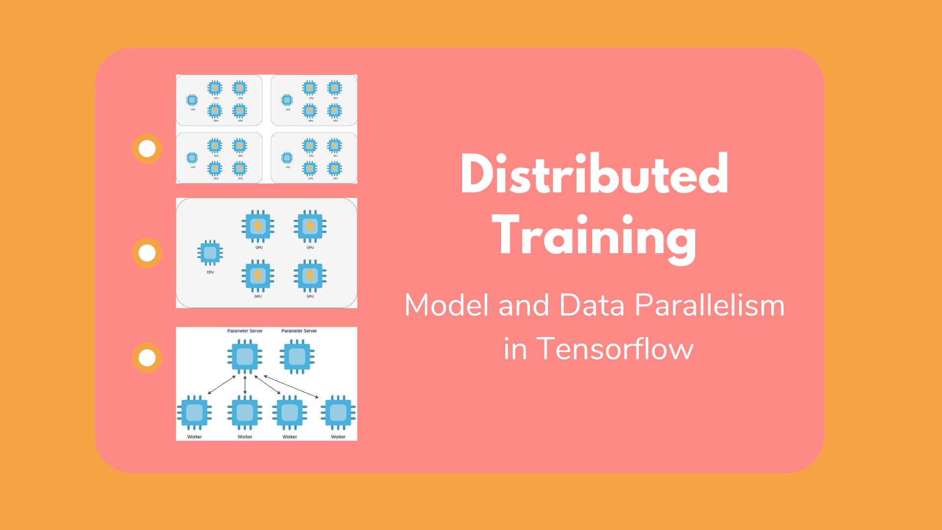
Data and Model Parallelism

The two major schools on distributed training are data parallelism and model parallelism.

In the first scenario, we scatter our data throughout a set of GPUs or machines and we perform the training loops in all of them either synchronously or asynchronously (you will understand what this means later). I would dare to say that 95% of all trainings are done using this concept.

Of course, it heavily depends on the network speed as there is a lot of communication between clusters and GPUs but most of the time is the ideal solution. Its advantages include things like: a) universality because we can use it for every model and every cluster, b) fast compilation because the software is written to perform specifically on that single cluster and c) full utilization of hardware. And to give you a preview, the vast majority of the remaining article will be focused on data instead of model parallelization. However, there are cases that the model is too big to fit in a single machine. Then model parallelism might be a better idea.

Model parallelism: enables us to split our model into different chunks and train each chunk into a different machine.

The most frequent use case is modern natural language processing models such as GPT-2 and GPT-3, which contain billions of parameters (GPT-2 has in fact 1.5 billion parameters).

Training in a single machine

Before we continue let's pause a minute and remind ourselves what training in a single machine with a single GPU looks like. Let's imagine that we have a simple neural network with two layers and three nodes in each layer. Each node has its own weights and biases, our trainable parameters. A training step begins with preprocessing our data. We then feed them into our network and it predicts the output (forward pass). We then compare the prediction with the desired label by computing the loss, and in the backward pass we will compute the gradients and update the weights based on the gradients. And repeat.

In the easiest scenario, a single CPU with multiple cores is enough to support the training. Keep in mind that we can also take advantage of multithreading. To speed things even more, we add a GPU accelerator and we transfer our data and gradients back and forth from the CPU’s memory to GPUs. The next step is to add multiple GPUs and finally to have multiple machines with multiple GPUs on each one, all connected over a network.

To make sure that we are all on the same page let's define some basic notations:

Worker: a separate machine that contains a CPU and one or more GPUs
Accelerator: a single GPU (or TPU)
All-reduce: a distributed algorithm that aggregates all the trainable parameters from different workers or accelerators. I’m not gonna go into details on how it works but essentially, it receives the weights from all workers and performs some sort of aggregation on them to compute the final weights.

Since most strategies apply on both worker and accelerator level, you may see me use a notation like workers/accelerators. This indicates that the distribution may happen between different machines or different GPUs. Equivalently, we can use the word Device. So those terms will be used indistinguishably.

Cool. Now that we know our basics it's time to proceed with the different strategies we can use for Data Parallelism.

Distributed training strategies

We can roughly distinguish the strategies into basically two big categories: synchronous (sync) and asynchronous.

In sync training, all workers/accelerators train over different slices of input data and aggregate the gradients in each step. In async training, all workers/accelerators are independently trained over the input data and update variables in an asynchronous manner.

Duh... Thank you Sherlock...OK let's clarify those up.

Synchronous training

In sync training, we send different slices of data into each worker/accelerator. Each device has a full replica of the model and it is trained only on a part of the data. The forward pass begins at the same time in all of them. They all compute a different output and gradients.

At this moment all the devices are communicating with each other and they are aggregating the gradients using the all-reduce algorithm I mentioned before. When the gradients are combined, they are sent back to all of the devices. And each device continues with the backward pass, updating the local copy of the weights normally. The next forward past doesn't begin until all the variables are updated. And that’s why it is synchronous. At each point in time, all the devices have the exact same weights, although they produced different gradients because they trained on different data but updated from all the data.

Tensorflow refers to this strategy as mirrored strategy and it supports two different types. The “tf.distribute.MirroredStrategy” is designed to run on many accelerators in the same worker while we “tf.distribute.experimental.MultiWorkerMirroredStrategy” is for use on multiple workers as you may have guessed. The basic principles behind the two of them are exactly the same

Let's see some code. If you remember, our custom training loop consists of two functions, the “train” function and the “train_step” function. The first one iterates over the number of epochs and runs the “train_step” on each one, while the second performs a single pass on one batch of data.

def train_step(self, batch):
        trainable_variables = self.model.trainable_variables
        inputs, labels = batch
        with tf.GradientTape() as tape:
            predictions = self.model(inputs)
            step_loss = self.loss_fn(labels, predictions)

        grads = tape.gradient(step_loss, trainable_variables)
        self.optimizer.apply_gradients(zip(grads, trainable_variables))

        return step_loss, predictions

   def train(self):
        for epoch in range(self.epoches):
            for step, training_batch in enumerate(self.input):
                step_loss, predictions = self.train_step(training_batch)

However, because distributing our training using a custom training loop is not that straightforward and it requires us to use some special functions to aggregate losses and gradients, I will use the classic high-level Keras APIs. Besides, our goal in this article is to outline the concepts rather than to focus on the actual code and the Tensorflow intricacies. If you want more details on how to do that, check out the original docs.

So, when you think of the training code, you will imagine something like this:

def train(self):
    """Compiles and trains the model"""
    self.model.compile(optimizer=self.config.train.optimizer.type,
                    loss=tf.keras.losses.SparseCategoricalCrossentropy(from_logits=True),
                    metrics=self.config.train.metrics)

    model_history = self.model.fit(self.train_dataset, epochs=self.epoches,
                                    steps_per_epoch=self.steps_per_epoch,
                                    validation_steps=self.validation_steps,
                                    validation_data=self.test_dataset)

    return model_history.history['loss'], model_history.history['val_loss']

And for building our Unet model, we had:

self.model = tf.keras.Model(inputs=inputs, outputs=x)

Check out the full code in our Github repo

Mirrored Strategy

According to Tensorflow docs: “Each variable in the model is mirrored across all the replicas. Together, these variables form a single conceptual variable called MirroredVariable. These variables are kept in sync with each other by applying identical updates.” I guess that explains the name.

We can initialize it by writing:

mirrored_strategy = tf.distribute.MirroredStrategy(devices=["/gpu:0", "/gpu:1"])

As you may have guessed we will run the training in two GPU's, which are passed as arguments inside the class. Then all we have to do is wrap or code with the strategy like below:

with mirrored_strategy.scope():
        self.model = tf.keras.Model(inputs=inputs, outputs=x)
        self.model.compile(...)
        self.model.fit(...)

The “scope()” makes sure that all variables are mirrored in all of our devices and that the block underneath is distribution-aware.

Multi Worker Mirrored Strategy

Similarly to MirroredStrategy, MultiWorkerMirroredStrategy implements training on many workers. Again, it creates copies of all variables across all workers and runs the training in a sync manner.

This time we use json configs to define our workers:

os.environ["TF_CONFIG"] = json.dumps(
    {
        "cluster":{
            "worker": ["host1:port", "host2:port", "host3:port"]
        },
        "task":{
            "type": "worker",
            "index": 1
        }
    }
)

The rest are exactly the same:

multi_worker_mirrored_strategy = tf.distribute.experimental.MultiWorkerMirroredStrategy()
with multi_worker_mirrored_strategy.scope():
    self.model = tf.keras.Model(inputs=inputs, outputs=x)
    self.model.compile(...)
    self.model.fit(...)

Central Storage Strategy

Another strategy that is worth mentioning, is the central storage strategy. This approach applies only to environments when we have a single machine with multiple GPUs. When our GPU’s might not be able to store the entire model, we designate the CPU as our central storage unit which holds the global state of the model. To this end, the variables are not mirrored into the different devices but they are all in the CPU.

Therefore the CPU sends the variables to the GPU's which perform the training, compute the gradients, update the weights and send them back to the CPU which combines them using a reduce operation.

central_storage_strategy = tf.distribute.experimental.CentralStorageStrategy()

Asynchronous training

Synchronous training has a lot of advantages but it can be kind of hard to scale. Furthermore, it may result in the workers staying idle for a long time. If the workers differ on capability, are down for maintenance, or have different priorities, then an async approach might be a better choice because workers won’t wait on each other.

A good rule of thumb, that, of course, isn’t applicable in all cases, is:

If we have many small, unreliable and with limited capabilities devices, it's better to use an async approach
On the other hand, if we have strong devices with powerful communication links, a synchronous approach might be a better choice.

Let's now clarify how async training works in simple terms.

The difference from sync training is that the workers are executing the training of the model at different rates and each one of them doesn't need to wait for the others. But how do we accomplish that?

Parameter Server Strategy

The most dominant technique is called Parameter Server Strategy. When having a cluster of workers, we can assign a different role to each one. In other words, we designate some devices to act as parameter servers and the rest as training workers.

Parameter servers: The servers hold the parameters of our model and are responsible for updating them (global state of our model).

Training workers: they run the actual training loop and produce the gradients and the loss from the data.

So here is the complete flow:

We again replicate the model in all of our workers.
Each training worker fetches the parameters from the parameter servers
Performs a training loop.
Once the worker is done, it sends the gradients back to all the parameter servers which update the model weights.

As you may be able to tell, this allows us to run the training independently in each worker, and scale it across many of them. In TensoFlow it looks something like this:

ps_strategy = tf.distribute.experimental.ParameterServerStrategy()
parameter_server_strategy = tf.distribute.experimental.ParameterServerStrategy()

os.environ["TF_CONFIG"] = json.dumps(
    {
        "cluster": {
            "worker": ["host1:port", "host2:port", "host3:port"],
            "ps":  ["host4:port", "host5:port"]
        },
        "task": {
            "type": "worker",
            "index": 1
        }
    }
)

Model Parallelism

So far, we talked about how to distribute our data and train the model in multiple devices with different chunks. However, can't we split the model architecture instead of the data? Actually, that's exactly what model parallelism is. Although harder to implement, it’s definitely worth mentioning.

When a model is so big that it doesn't fit in the memory of a single device, we can divide it into different parts, distribute them across multiple machines and train each one of them independently using the same data.

An intuitive example might be to train each layer of a neural network in a different device. Or perhaps in an encoder-decoder architecture to train the decoder and the encoder into different machines.

Keep in mind that in 95% of the cases the GPU has actually enough memory to fit their entire model

Let's examine a very simple example to make that perfectly clear. Imagine that we have a simple neural network with an input layer, a hidden layer, and an output layer.

And the hidden layer might consist of 10 nodes. A good way to parallelize our model would be to train the first 5 nodes of the hidden layer into one machine and the next 5 nodes into a different machine. Yeah, I know it’s an overkill for sure, but for example’s sake let's go with it.

We feed the exact same batch of data into both machines
We train each part of the model separately,
We combine the actual gradients using an all-reduce approach as in data parallelism.
We run the backward pass of the backpropagation algorithm in both machines
And finally we update the weights based on the aggregated gradients.

Notice that the first machine will update only the first half of the weights while the second machine the second half.

As I mentioned before in the article the most common use case of model parallelism is natural language processing models such as Transformers, GPT-2, BERT, etc. In fact, in some applications engineers combine data parallelism and model parallelism to train those models as fast and as efficiently as possible. Which reminds me that there is actually a TensorFlow library that tries to alleviate the pain of splitting models called Tensorflow Mesh (be sure to check it out if you are interested in the topic). I'm not going to dive deeper here because to be honest with you I haven't really needed so far to use model parallelism and probably most of us won't ( at least in the near future).

As a side material, I strongly suggest the TensorFlow: Advanced Techniques Specialization course by deeplearning.ai hosted on Coursera, which will give you a foundational understanding on Tensorflow

Conclusion

In this article, we finally summed up the training part of our deep learning in production series. We discovered how to write a custom high-performant training loop in TensorFlowThen we saw how to run a training job in the cloud. Lastly, we explored all the different techniques to distribute the training in multiple devices using data and model parallelism. I hope that by now you have a very good understanding of how to train your machine learning model efficiently.

We are at the point where we built our data pipeline and we trained our model. Now what?

I think it's time to use our trained model to serve users and provide them with the ability to perform image segmentation into their own images using our custom UNet model.

To give you a sneak peek of the following articles, here are some topics we're gonna cover in the next articles:

APIs using Flask
Serving using uWsgi and Nginx
Containerizing Deep Learning using Docker
Deploying application in the cloud
Scaling using Kubernetes

If I triggered your interest even slightly, don't forget to subscribe to our newsletter to stay up-to-date with all of our recent content. That’s all I had for now.

To be continued...

References

* Disclosure: Please note that some of the links above might be affiliate links, and at no additional cost to you, we will earn a commission if you decide to make a purchase after clicking through.